9 Perturbations within Projections
9.1 Introduction
Within the simulation framework used in aMSE, the population dynamics are not deterministic and variation is introduced in the projections through random variation in the predicted recruitment levels, through variation being introduced in the how the actual catches are distributed among the populations (essentially this is in teh description of the fleet dynamics), and finally, with variation being introduced into the expression of the predicted cpue from the dynamics (this latter is important as all the current harvest strategy performance measures are based upon the commercial cpue).
There are other sources of change and variation that are not accounted for. It is known that there have been marine heatwave events that have led to mortality events observed by divers (exceptional numbers of dead abalone shells washing back and forth in gutters). Such events have been confirmed to correspond to observed oceanographic events entailing large deviations from average sea temperatures. The effects of such heatwaves, destructive storm events, and other external occurrences, such as toxic algal blooms, are not known from direct observations except for the anecdotal observations from divers. These observations inform that there has been an impact but provide no measure of the extent or severity of any such impacts. When we apply a stock assessment model, such as that implemented in the sizemod R package, effectively the dynamics as described by such models only identifies the catches and recruitment deviates as the only drivers of the observed dynamics. Without real data on possible impacts due to environmental events their scale of any impact cannot be estimated.
In Australia, there have been heatwave events whose impact is undeniable. In Western Australia, during 2011?, a significant heatwave event occurred down the west coast with one of its impacts being the effective elimination of the Haliotis roie stocks north of Perth. Other, less severe heatwave events (and other such perturbations) potentially can have impacts on survivorship of both the emergent and the cryptic animals currently alive. In addition, it is simple to imagine that the physiological shocks experienced by mature animals may well reduce recruitment success rather than induce death (i.e. sublethal effects). Given these considerations a need has therefore been identified for having a facility within aMSE for exploring the longer-term influence of possible perturbations to survivorship of currently settled animals but also of perturbations to recruitment success in selected years. The simulation framework is designed to explore the performance of different versions of abalone harvest strategies. It is expected that marine heatwaves and other such perturbations will occur into the future, so it will be valuable to be able to determine how each tentative harvest strategy handles the possible outcomes of significant perturbations to either survivorship or recruitment, or both.
9.2 Methods and Results
The capacity to introduce perturbations into the recruitment and the survivorship of post-larval animals has been introduced in such a way that no changes are required if no perturbations are wanted in a set of simulations. Thus, only if perturbations are required are changed required, and the only changes required involve adding a few lines of detail into the control file, which every scenario must have. No changes are required to any other files.
In the control file major sections are identified by capitalized headings such as ‘START’, ZONE’, ‘RECRUIT’, and ‘RANDOM’. The new section can go anywhere but it is proposed that when it is wanted it gets introduced between the ‘PROJECT’ and the ‘PROJLML’ sections. Thus, in a control file with no defined perturbations one might have:
…
initLML, 140, initial LML for the unfished zone if no historical catches used
PROJECT, 30, number of projection years for each simulation
PROJLML, need the same number as there are projection years
2021, 145, Legal Minimum Length (LML, MLL, MLS) e.g. 140
2022 , 145
…
9.2.1 ENVIRON
To add a single year of perturbations we can add:
…
initLML, 140, initial LML for the unfished zone if no historical catches used
PROJECT, 30, number of projection years for each simulation
ENVIRON, 1, numbers of years of intervention
eyr, 5, which projection years will have an event
proprec1, 0.3, 0.3, 0.3, 0.3, 0.3, 0.3, 0.3, 0.3, one for each sau
propNt1, 0.99, 0.99, 0.99, 0.99, 0.99, 0.99, 0.99, 0.99, one for each sau
PROJLML, need the same number as there are projection years
2021, 145, Legal Minimum Length (LML, MLL, MLS) e.g. 140
2022 , 145
…
The new keyword is ‘ENVIRON’. The commas are important as they identify the separate fields that aMSE needs to read.
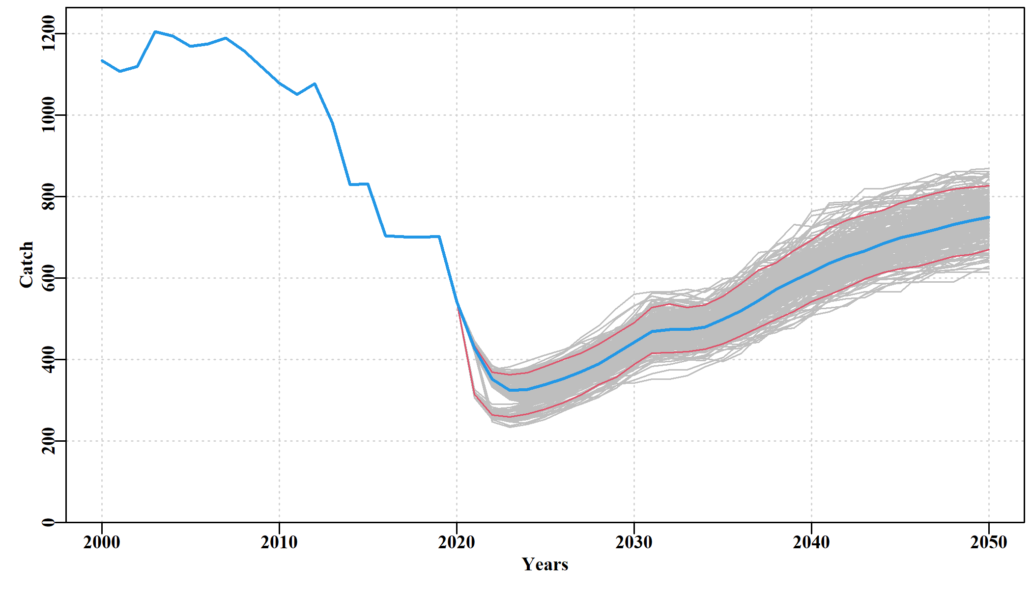
This set up would impose a perturbation in the fifth projection year and the impact will force the recruitment to be only 0.3 of the predicted recruitment level taken off the deterministic stock-recruitment curve for each population, when it only had 10 percent of the usual random recruitment variation that every other year experiences. Survivorship of post-larval animals will be 99 percent, so only a tiny impact on emergent and cryptic animals. If once this section has been introduced, one wants to turn off the perturbation then all that is needed is to set the ‘ENVIRON’ number = 0. That number must be greater than zero for there to be an effect.
With almost no impact on settled individuals the outcome on the dynamics only becomes apparent after a delay of between 5 - 8 years.
To add two years in which perturbations occur we can add:
…
initLML, 140, initial LML for the unfished zone if no historical catches used
PROJECT, 30, number of projection years for each simulation
ENVIRON, 2, numbers of years of intervention
eyr, 5, 8, which projection years will have an event
proprec1, 0.3, 0.3, 0.3, 0.3, 0.3, 0.3, 0.3, 0.3, one for each sau
proprec2, 0.3, 0.3, 0.3, 0.3, 0.3, 0.3, 0.3, 0.3, one for each sau
propNt1, 0.99, 0.99, 0.99, 0.99, 0.99, 0.99, 0.99, 0.99, one for each sau
propNt1, 0.99, 0.99, 0.99, 0.99, 0.99, 0.99, 0.99, 0.99, one for each sau
PROJLML, need the same number as there are projection years
2021, 145, Legal Minimum Length (LML, MLL, MLS) e.g. 140
2022 , 145
…
which gives rise to:
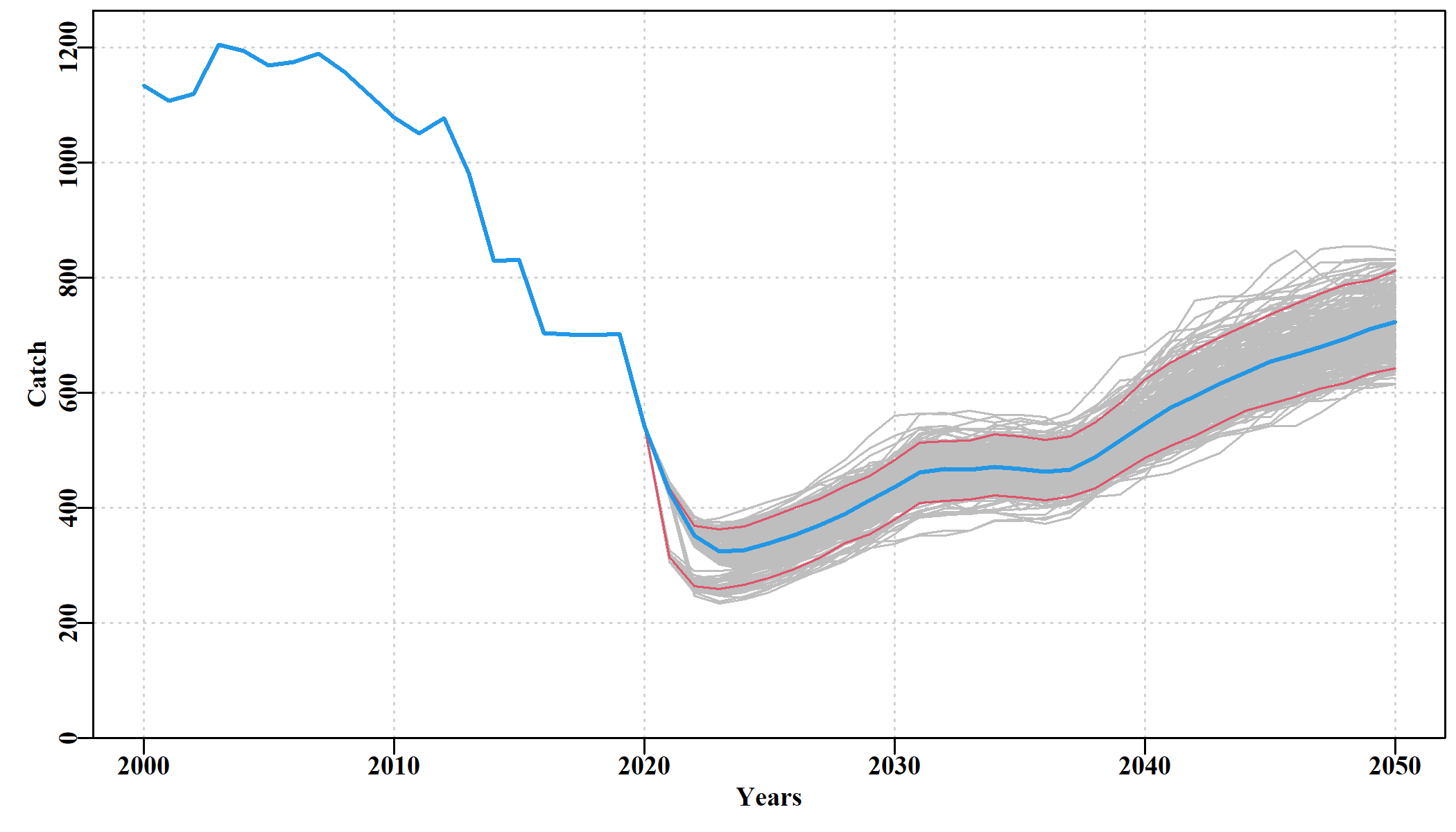
When the results of these perturbations are compared with the identical harvest strategy with no perturbations then the impacts become clearer.
9.2.2 TIMEVARY
A more recent perturbation keyword is TIMEVARY. This has been implemented to allow for time trends in biological factors relating to productivity. Initially, this is limited to recruitment levels only but may become extended to cover such things as time-varying growth and or maturity.
As with the ENVIRON keyword, if it is completely omitted from the control file , or its initial setting set = 0, then it will be ignored and will have no effect. Thus, no changes are required to any control files that currently work as they are intended. Without time-varying recruitment then recruitment during projections is simply the expected recruitment off the stock recruitment curve with either known recruitment deviates included or with Log-Normal variation, the scale of which is controlled with the withsigR parameter. This might be considered the standard recruitment. The advent of the time-varying recruitment option means that through the projections the standard recruitment that would normally occur is multiplied by a given proportion in a given year. One sets the starting proportion (usually = 1.0, meaning go with the standard recruitment level), and the second parameter is the proportion of the standard recruitment that is expressed in the final projection year. The outcome for setting up a set of time-varying recruitment levels is currently limited to arranging a linear change of the proportion of the expected standard recruitment level. The format in the control file would be:
TIMEVARY,1,,
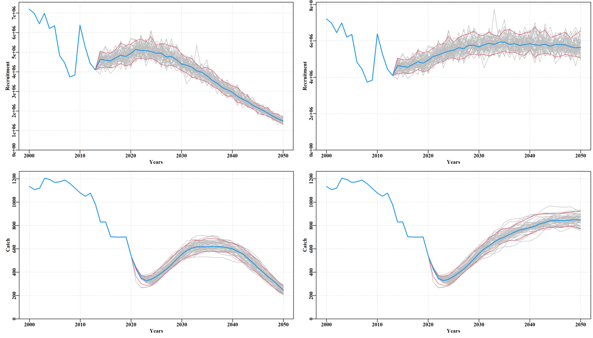
deltarec,0.3,,This would imply a linear decline from a multiplier on the standard recruitment in the projection years from 1.0 : 0.3 across the projection years. This would imply a 70% drop in productivity across the years of projection. Such a decline would push the Tasmanian harvest strategy to invoke a very large drop in catches but this would not be sufficient to reverse the decline because in this case, the decline is literally a decline in productivity rather than an impact of the fishery.
If the effect of such a, hopefully, badly exaggerated, change is compared to the expected dynamics in the absence of such a decline, the impacts become clear.
9.3 Comparing Scenarios
It should be clear that if a sequence of environmentally driven perturbations occur that significantly disrupt the recruitment success, then the stock recovery will be compromised. Given the increasing frequency of such events as marine heat waves, and the slow rise in local sea temperatures, such changes are a real possibility that needs to be included in any considerations given to rebuilding abalone stocks.
Given the availability of this facility to introduce perturbations it is now possible to explore how large a perturbation must be to have a significant impact (the example of repeated zone-wide 70% reductions in recruitment success would constitute quite a severe impact). Now it is possible to examine the effect of smaller scale events (at a scale of sau) on the potential risk to stock rebuilding.