2 Management Strategy Evaluation - MSE
2.1 The Need for Testing Alternative Management Options
Management Strategy Evaluation is used to compare and test different ways of managing exploited natural populations, especially in fisheries. MSE was developed as management of natural resources became more sophisticated (de la Mare, 1986; Smith, 1994; Punt et al, 2016). There were many years of using what turned out to be overly simplified objectives for commercial fisheries management, however, since about the mid-1990s (FAO, 1995, 1996, 1997) there has been a growing trend of explicitly defining a fishery management policy to be used in each jurisdiction, Such policies are different from a Fisheries Management Plan and generally, they explicitly address issues relating to sustainability, managing risk factors, managing bycatch, and actions relating to threatened and endangered species. This is an important improvement over vague exhortations to achieve the maximum sustainable yield for each species without defining what aspect of MSY was the traget or how to achieve that.
In addition to explicit statements defining management objectives, there was/is a move to introduce explicit and formal harvest strategies aimed at how to manage each fishery so as to achieve those objectives. Such formal ‘harvest strategies’ were first put together for the larger, more valuable fisheries that already had detailed integrated stock assessment models describing their dynamics. Such models led to the development of harvest strategies that involved a feedback mechanism that responded to the stock status, most often depletion level, relative to limit and target reference points of estimated depletion. However, not all species are amenable to the use of the formal mathematical models used to determine stock depletion levels. In such cases it is still possible to develop a formal yet empirical harvest strategy. This is the case with many hard to age, and especially highly spatially structured stocks, such as found with abalone, beche de mer, and other small scale coastal fisheries targeting relatively sedentary species (the S-fisheries of Parma et al 2003; Oresanz et al, 2005). There are many possible approaches to developing empirical harvest strategies, with no, as yet, clearly preferred approaches. Unfortunately, unintended consequences are not uncommon when attempting to control or manage relatively complex natural systems with a set of rules, so, generally, to avoid potentially disastrous outcomes, it is best to test and compare any new versions of an EHS and the candidate alternative management arrangements before implementing them.
Comparing the relative effectiveness of alternative harvest strategies for particular fisheries generally requires the use of Management Strategy Evaluation (Smith, 1994; Punt et al. 2001; Haddon, 2007; Punt et al. 2016).
2.1.1 How Does MSE Work?
As stated by Punt et al. (2016, p303): “Management strategy evaluation (MSE) involves using simulation to compare the relative effectiveness for achieving management objectives of different combinations of data collection schemes, methods of analysis, and subsequent processes leading to management actions. MSE can be used to identify a ‘best’ management strategy among a set of candidate strategies, or to determine how well an existing strategy performs. The ability of MSE to facilitate fisheries management achieving its aims depends on how well uncertainty is represented, and how effectively the results of simulations are summarized and presented to the decision-makers. Key challenges for effective use of MSE therefore include characterizing objectives and uncertainty, assigning plausibility ranks to the trials considered, and working with decision makers to interpret and implement the results of the MSE.”
Note there is potential for confusion between the terms management strategy, management procedure, and harvest strategy. Such potential confusion brought about by different terms being used for the same or similar concepts is a common problem in fisheries science. Even though historically the term ‘harvest strategy was first used to describe the three classic strategies of ’constant catch’, ‘constant fishing mortality’, and ‘constant escapement’, the term ‘harvest strategy’ has come to replace ‘management strategy’ so, here, we will attempt to consistently use the term ‘harvest strategy’. The fact that that last sentence is confusing reinforces the notion that the focus should be on combinations of 1) data collected and used, 2) analysis or assessment of that data, and 3) a harvest control rule that uses the results of parts 1 an 2, to determine the recommended management advice.Give a particular setup, a change in any one of those three would strictly constitute a different harvest strategy to the original.
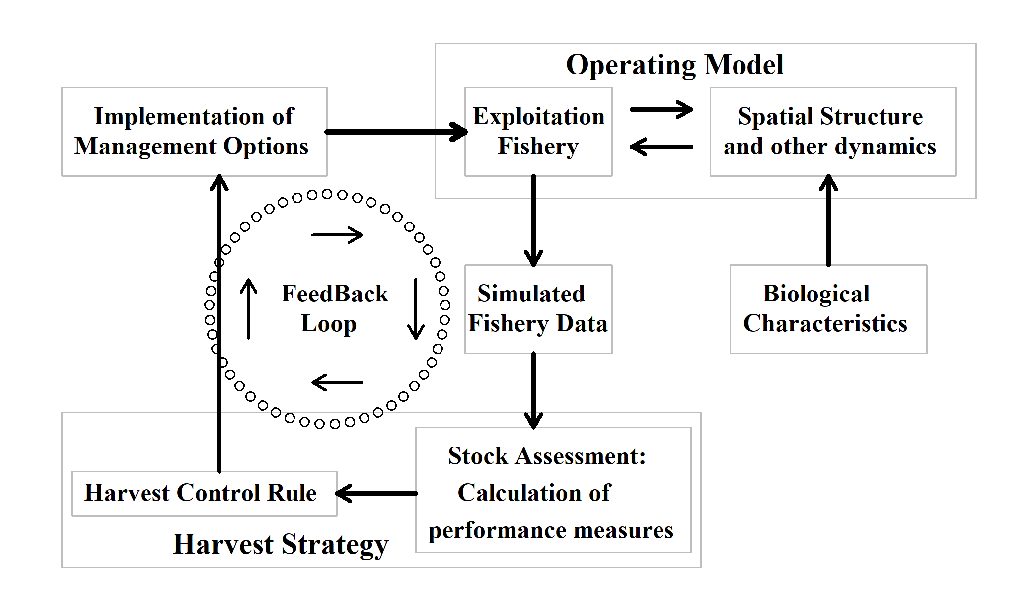
The simulations within MSE involve using a mathematical model to mimic both the biological and fishery/fleet dynamics of the fishery being considered. This simulation model is usually termed the Operating Model or OM. It is possible to use a relatively standard assessment model as an OM in which case it could be fitted directly to data from a real fishery. It would be uncommon, but not impossible to use such an approach to test different harvest strategies within a fishery being assessed by the same model. It is more common to use a rather more complex model of a system than any of the assessment models used to assess a stock. This is necessary so that the robustness of any selected ‘harvest strategy’ can be tested when the assessment’s assumptions about spatial structure, or population dynamics, or some other structural assumption, are incorrect. A more complex OM than the assessments used can provide multiple scenarios to enable the simulations to determine how the simpler model responds when the ‘reality’ from which the observed data are derived differs from the ’reality implied by the assessment’s assumptions and structure. Such more complex models can only be conditioned (its parameters adjusted) until its dynamic behaviour reflects the observed properties of a real fishery. Once appropriately conditioned (easily stated, not necessarily simple to do), the dynamic behaviour of the operating model is taken to represent reality and is used to simulate the operation of a fishery under the different harvest strategies (HS) being compared or tested (see Dichmont et al 2006; Dichmont and Brown, 2010; Haddon et al, 2003; Haddon and Mundy, 2016).
The essential aspect of such a simulation, that makes an MSE differ from a standard forward projection of a stock assessment under constant catch or effort (a classical risk assessment; Francis, 1992; Francis and Shotton, 1997), is the built-in feedback of the regular management advice into the dynamics described by the operating model. The importance of a feedback mechanism between the dynamics and the management advice has been recognized from the early days of MSE (de la Mare, 1986). The dynamics of the stock and fishery are simulated each year, the HS (data sampling, assessment/analysis, and harvest control rule) is applied however often the HS dictates, and the outcome of the specific HS is fed back into the operating model as a Total Allowable Catch or Effort, or some other management influence. Such inputs could be expected to alter the path of the expected dynamics (this constitutes the feedback loop). In this way, different HS can be expected to have different simulation outcomes over a set number of years (see Figure 2.1).
It is also important to note that not all management strategy evaluations involve simulating a real fishery. There are many general questions that can be answered using hypothetical fishery situations rather than simulating a specific fishery. Some examples used in the documentation of the aMSE MSE code-base use only a portion of a real fishery, which is a mixture of realistic and unrealistic (because in reality the fleet dynamics used relates to a whole quota zone not just one or two sau - spatial assessment units). Nevertheless, such hypothetical situations can be used to explore the influence of different sources of uncertainty on differing harvest strategies.
2.1.2 Simpler is Not Necessarily Better
The MSE process is often represented in an overly simplistic fashion leading to un-realistic expectations as in: ‘if a given harvest strategy has been MSE tested, and nothing untoward found, then it must be good’. However, it is important to remember that, as with any model, if an operating model does not include a particular feature in its dynamics (e.g. does not include depensation in its recruitment dynamics, or non-linearity in the relationship between stock biomass and CPUE, the latter is included in aMSE) then the effectts of those features can, obviously, never be expressed or tested in the simulations. The structure of an operating model needs to be well documented, and its limitations understood, so that the domain of applicability the MSE testing for each HS is known. This is especially important to understand because harvest strategies that have been MSE tested are generally held in relatively high regard. However, the completeness of any MSE testing will always be constrained to the dynamics described by the operating model, so care in its design is required and that design needs to be defensible (see Operating Model Structure in teh aMSEGuide).
2.1.3 Harvest Strategies
In the literature a harvest strategy (Smith, 1997; Haddon, 2007), or HS, aimed at achieving a defined policy objective, has a minimum of three components:
Specified and representative data collected from the fishery being evaluated,
An assessment or analysis of the fishery, based on the data collected, that estimates its status relative to pre-defined target and limit reference points,
A formal harvest control rule (decision rule) that defines previously agreed management advice (future catch or effort levels, etc) in response to a stock’s status relative to its reference points.
Each of the three components can be varied in multiple ways and, strictly, each such combination would constitute a different harvest strategy (HS). Therefore, for any fishery, there will be multiple potential options available for the management. Often, fishery management involves balancing trade-offs between conflicting objectives. For example, with a valuable species such as abalone (e.g. blacklip abalone, Haliotis rubra) the two objectives of maintaining a sustainable stock and maximizing the profitable catch are potentially in conflict, or at least can be when considered across different time-frames. Such potential conflicts within fisheries was one reason why management strategy evaluation was developed to enable the comparison of how alternative harvest strategies perform relative to different objectives. MSE methods originated in the International Whaling Commission (de la Mare, 1986), which had its own contentious issues (Punt and Donavan, 2007). It is used to select or develop an optimum HS, or at least reject sub-optimal ones.
2.1.4 Management Strategy Evaluation of Abalone Fisheries
There have been previous attempts to conduct management strategy evaluation (MSE) of alternative harvest strategies for abalone fisheries in Australia (Haddon et al., 2013; Haddon and Helidoniotis, 2013; Haddon and Mundy, 2016). In the current project, an R package aMSE (Haddon, 2025) has evolved and has been developed from those earlier attempts (Haddon, 2025a). Other complementary R packages (codeutils, hplot, makehtml, and sizemod, (Haddon, 2025b, c, d, e), each with their own documentation) have also been generated or modified from earlier versions to assist with conditioning the operating model within the MSE, and the production of a standard set of summary figures and model information.
An example R package EGHS has been developed that implements a simpler version of the Tasmanian abalone harvest strategy in a manner useful for the examples described in the aMSEGuide (Haddon & Mundy, 2024b). Ideally, each jurisdiction that uses aMSE would encapsulate their own harvest strategies into such a package, as this simplifies maintenance as well as the use of aMSE. The required documentation within each formal R package for an HS, and the possibility of including a vignette with more details, means that the workings of the HS in each case could be explained and made clear. A formal package avoids the possibility of source files of R functions being modified such that different users inadvertently end up using a different HS structure. Maintenance and possible developments within the code can also be managed more effectively when it is structured as a formal package.
The R code in the aMSE package is a greatly developed and translated version of the relatively undocumented Abalone MSE code developed and used in Haddon et al (2013), which had been developed further, but with only slightly better documentation, in Haddon and Mundy (2016). The essential equations describing the operating model dynamics used in those earlier projects were formally published in Haddon and Helidoniotis (2013). Those dynamics have since been found to be overly complex in that they used separate vectors of numbers-at-length to describe the cryptic and emergent components of each of the many abalone populations simulated to make up a simulated quota zone. Other, unpublished, work demonstrated that this separation has no real advantages for representing the stock dynamics but does have serious computational disadvantages. The new aMSE package reflects this by changing the previous equations so they now use only a single vector of numbers-at-length to contain the dynamics for each year. In addition, other methods are being incrementally implemented with the intent of speeding the computations. Previously, it could take hours to appropriately explore even a single HS, which now, depending on the complexity of the HS, can take only minutes to run a single scenario made up of several hundred replicate runs.
The underlying objective in the current aMSE R package is to enable the simulations and MSE testing of different HS to proceed by users familiar with R, but without months of introductory training with the bare software code-base, as needed previously. This document is a first attempt to provide the background required for others to successfully run the software. While writing this material, sections will be borrowed freely from both Haddon et al (2013) and Haddon and Mundy (2016), wherever it is appropriate. These two projects, in which abalone MSE code was first developed, did not include sufficient time or resources to generate a more user-friendly or documented code-base for the software. Relatively user-friendly software improves the capacity of other fisheries assessment scientists to apply these methods to more stocks or to new HS currently being developed. By making the new R package open-source, freely available, and fully documented, the intent and hope is that more people will find the methods workable. By being defined within open-source software this also allows for future developments of the package by others should they wish. One primary objective is to allow users to write their own functions or R packages describing any new harvest strategy, or figure, or table, that they might develop.
2.1.5 Difficulties Inherent with MSE Testing Abalone HS
The phrase ‘abalone stock’ sounds meaningful and most would consider this to refer to the standard notion of populations of a species having sufficient genetic homogeneity to represent a connected reproductive whole. However, as demonstrated by Miller et al (2009; 2014), genetic studies indicate that abalone populations (at least of blacklip and greenlip abalone) are meta-populations made up of multiple, what might be termed, micro-stocks. Such micro-stocks are functionally independent, while remaining genetically connected such that divergence is not occurring In effect, the management areas for which total allowable catches (TACs) and minimum legal sizes (MLS or LML) are set are spatially recognizable and convenient areas or zones that are composed of numerous mostly isolated micro-stocks. The solution adopted in Haddon et al (2013) and Haddon and Mundy (2016) was to generate an operating model made up of numerous discrete populations of abalone, each with their own set of biological properties and fishery productivity that reflected properties observed within real fisheries. One disadvantage of this approach was that there was no chance of fitting this model to a real fishery as no real fishery has sufficient data available concerning differences in growth, size-at-maturity, and other matters relating to productivity. This meant that one could only attempt to condition the operating model to have outputs and properties that approximately matched a real fishery. Of course, as those properties were defined at a large geographical scale there would be no single or unique way of setting up a large number of individual populations to mimic such emergent or sum-of-the-parts properties.
One time-consuming option to counter this problem would be to set up the operating model’s underlying populations in a number of ways to determine whether each different arrangement leads, effectively, to the same outcome. While this would be time-consuming it used to be the only way available of characterizing the full uncertainty relating to the spatial dynamics. There is now the possibility, however, that the use and collection of the GPS data-logger data can assist with the conditioning of the operating model, by allowing populations at a smaller scale to be more fully characterized, rather than at the scale of statistical reporting blocks within quota zones. Now there are 10+ years of such data in Tasmania, this database has now been used to define areas of persistent productivity (apps) that represent the multiple populations used to define the spatial assessment units (SAU) within the quota zone. Using the longer-term yield obtainable from each such smaller region as a proxy for their relative productivity provides an insight into the required dynamics from each of these ‘populations’ (or ‘areas of persistent production’, see Haddon, 2025b).
2.1.6 Applications in Victoria
During the research described in Haddon and Mundy (2016), an opportunity arose to apply that abalone MSE to some individual reefs within Western Victoria to examine how recovery might proceed under different harvest strategies following the viral destruction brought about by the AVG virus (Haddon & Helidoniotis, 2014). This differed from the applications in Tasmania as it was focussed solely on one reef complex, known as The Crags. While the operating model was still only conditioned on reality (rather than fitted) using the biological properties known for the abalone on The Crags, more time was spent improving the comparison of the length composition and historical performance of the fishery. This could be done by selecting combinations of simulated populations whose combined dynamics more closely followed trends in catches and size-composition through time. However, this process was very time-consuming, so the objectives of each study need to be made clear and explicit before embarking on such detailed conditioning.
2.1.7 Why is the Code so Specialized
To date, one reason that running an MSE remains relatively specialized and esoteric is that the simulation framework needs to be able to simulate a wide range of processes (see Figure 2.1). These processes include a) the dynamics of the selected biological stock, b) the dynamics of the fishery imposed on the stock (the fleet dynamics), c) the generation of simulated fishery data from the fishery, d) the stock assessment or analysis applied to that data to estimate performance measures, and e) the control rule used to modify the present management options. For abalone this generally means changing the TAC, which is then fed back into the dynamics of the stock in a feedback loop within the modelling framework (Punt et al, 2016). In Tasmania, the TAC is the sum of the recommended aspirational catches in each SAU.
Developing and using such a complex software framework entails specialized expertise. The disadvantage of this is that it constrains its use with real fisheries and limits future developments. This is the primary reason for attempting to translate the MSE code into a documented R package. If more people can more easily take on the application of using the management strategy evaluation framework to explore management options for abalone stocks this should increase the chances of the adoption of improvements in management.
2.2 The Operating Model Structure
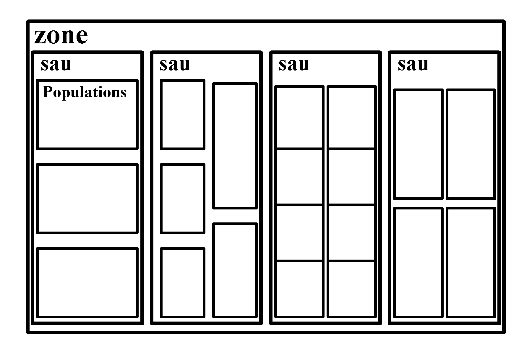
The operating model (OM) requires conditioning on a selected abalone fishery because the OM acts as a proxy for reality in the simulations. The task of the OM is to model the stock dynamics across all the micro-stocks embedded in the framework. Currently, a selected abalone fishery zone can have 10s or 100s of sub-populations, each with their own defined properties reflecting somewhat different growth, maturity, and other details relating to productivity (if GPS logger data is available then the persistent productivity of smaller areas within each SAU can be defined). However, such a simulation would be extremely complex to condition to a specific fishery simply because the data requirements would be enormous. To define the operating model within the MSE, the number of populations (numpop in the R code) need to be specified and how these are conditioned will, obviously, greatly influence the outcomes.
The original abalone MSE (Haddon et al, 2013) was designed for use with Tasmanian blacklip abalone stocks. Spatially this was structured as statistical blocks within quota zones. In Tasmania, quota zones were introduced from 2000 onward whereas the statistical blocks have been extant since 1965 (Anon, 1966). Biological data was available from many sites around Tasmania although it tended to be summarized at a block level. Each statistical block could be simulated as containing multiple populations (areas of persistent productivity), and each population has its own set of properties with many such properties relating to the productivity. To attempt to capture some of the between block variations in biological properties each block simulated was given its own set of average properties. These included, for many of the properties, a definition of a statistical distribution to describe the expected distribution of values across contained populations, for such things as the growth parameters, the parameters relating to maturity-at-size, and details of the stock recruitment relationship. Thus, each sub-set of populations (in Tasmania representing a statistical block but elsewhere they might represent any spatial assessment unit), was sampled from selected distributions that had been conditioned on what is known about the fishery being simulated. There is also the option of specifying particular values of the productivity parameters (growth, maturity, recruitment) for each ‘population’ (see the chapter on Conditioning on Populations in Haddon, 2025b).
Unfortunately, in fisheries management in general, and abalone fisheries in particular, the terminology used to describe different management details and concepts is not standardized across jurisdictions. Thus, while the term Zone is used widely to describe a geographical area over which a particular quota/TAC may be taken, the names given to sub-zones within zones differs between jurisdictions. The statistical block from Tasmania is not equivalent to the reef-code from Victoria, although it is closer to the spatial assessment unit from South Australia, though tends to be larger than the spatial management units in Central Victoria. Similarly, in Tasmania, the phrase the Legal Minimum Length (LML) is used to define legal size limits, which is equivalent to the Minimum Legal Length (MLL), and other such abbreviations from other jurisdictions. In aMSE we have used Zone for the largest scale of management, sau for the current spatial scale of assessment (sau can either be capitalized or not), and LML for the legal minimum length. When using the MSE, people in different jurisdictions should hopefully be able to manage any required translation without excessive indignation; it is the concept that matters not the word or phrase.
In an operational simulated zone different SAUs are likely to have different numbers of contained populations, and the populations are likely to be of very different sizes, each population with its own particular properties. Within the Tasmanian application of aMSE, the populations have been defined from the GPS data-logger information and are more akin to ‘areas of persistent productivity’.