While it would be possible to open the same tab in each of the three pages and step between them for a visual comparison that is not conducive to making useful comparisons. Instead, R functions have been generated that make a series of comparisons between the scenarios by first reading in the stored out objects from each MSE run. This involves knowing the outdir that was used and selecting those stored objects that contain the information about each scenario that the user wants to compare. So, assuming that a number of scenarios have already been run (as above), first we set up the required libraries and directories and then list the contents of outdir so an explicit selection can be made. If the user has setup a different way of storing their results then, obviously, a different way of selecting and reading the required scenarios will be required.
The Different Tabs
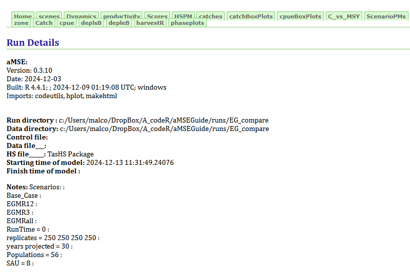
Hopefully, by now, it is not unexpected that the Home tab exhibits details relating to the run.
The comparisons begin in the scenes tab, which currently only contains a single table detailing the underlying characteristics of each scenario. This table is a repeat of the table of scenario characteristics printed to the console.
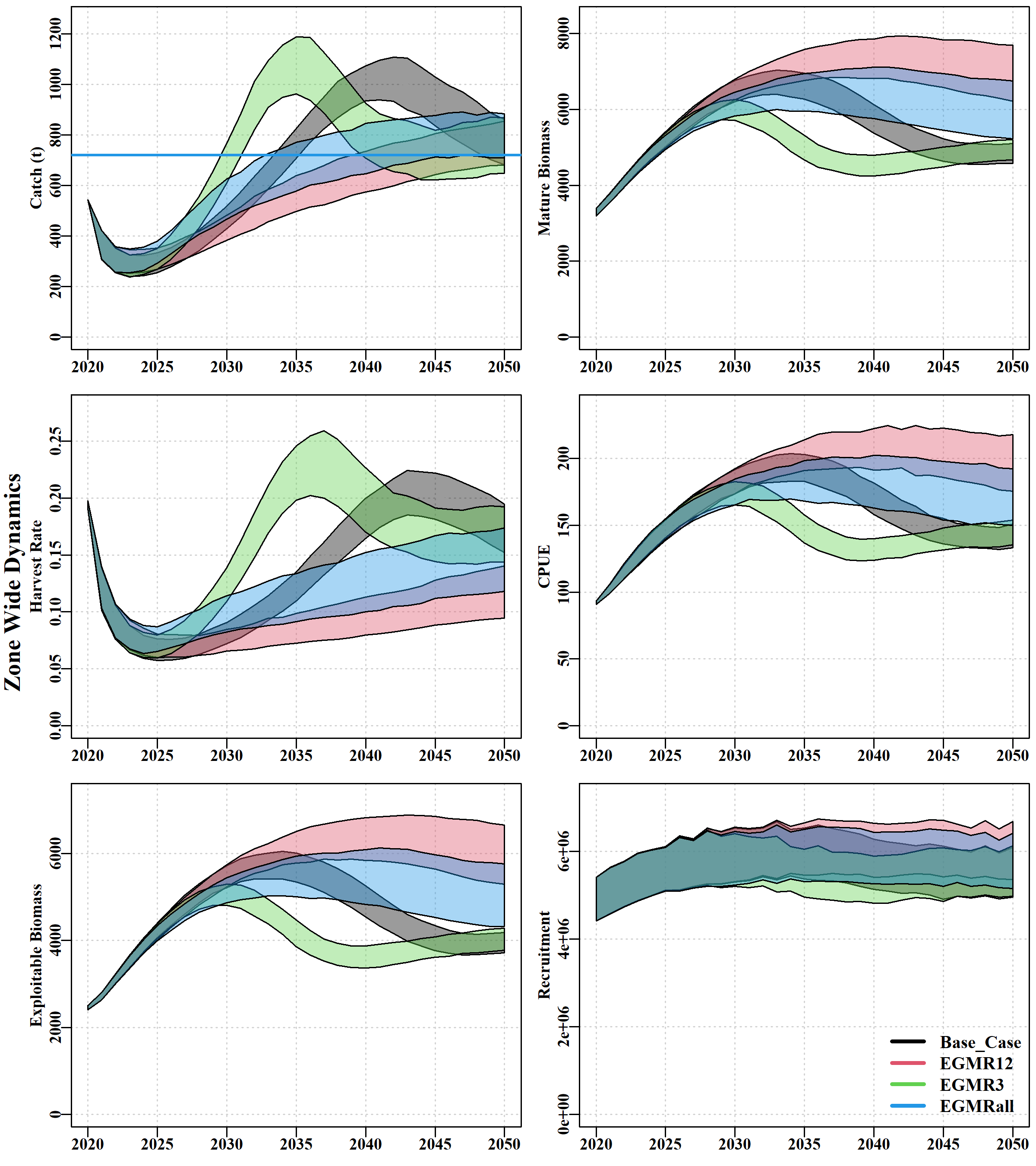
Given the challenge is to recover the stock in each SAU and that should allow the recovery of the fishery, a balance or trade-off is required between the rapidity with which catches are returned to the fishery and the rate at which stock biomass is predicted to recover. As the plots in the Dynamics tab demonstrate, returning catches too rapidly does not allow the biomass to increase as quickly, as evidenced by the predicted CPUE rising then falling rapidly. To approach a more stable and resilient fishery such oscillations are best avoided.
Dynamics tab, where the median and 90th quantiles of the predicted projections for cpue, actual catch, mature biomass, and harvest rate for each scenario are plotted against each other. Few differences occur between scenarios in their CPUE until between 2028 – 2030, depending on which Sau is considered. SAU 13 exhibits the relatively similar trends through time. In all other SAU the no meta-rule (noMR) and meta-rule 3 (MR3) scenarios exhibit a similar oscillatory trend except the noMR has a time-lag to reach the minimum CPUE of about 10-11 years. In all cases in all scenarios (except in SAU13) CPUE remains above 100kg following the period of stock recovery. The MRall appears to achieve a relatively stable CPUE more rapidly than MR12 and does not reach such high levels.
In terms of predicted catches MR3 returns catch to the fishery the fastest but then rapidly reduces it again to become more stable eventually. As with CPUE, noMR follows a similar pattern just 10 years more slowly. MRall leads to somewhat higher stable catches than MR12 and once again appears to find an improved balance between speed of recovery of the fishery and a conservative return of catches. These outcomes are reflected in the predicted annual harvest rates as well.
The mature biomass follows approximately the same trajectories in all scenarios until 2028-2030 where they begin to diverge. noMR and MR3 aer both oscillatory with noMR lagging behind the MR3. MR12 and MRall are both more stable in their trajectories with the MR12 scenario ending up with a somewhat higher level of mature biomass in all SAU except SAU13. While that is a positive thing for the stock it implies a somewhat lower final catch.
The Productivity tab only exhibits a single table, which implies that all scenarios share the same productivity characteristics. If the selected scenarios differed in some factor that influenced productivity (perhaps different natural mortality values) then each different scenario would have its own table of productivity properties by sau.
The Scores tab illustrates the final median harvest strategy scores for each sau and compare them in the plot. But each scenario has a table with the final scores tabulated. These data derive from functions within EGHS and will quite likely require changes when other Harvest Strategies are implemented. Given the harvest control rule implemented in the HS the median target would be a value of six (where values between 5 and 6 imply no change in catch).
The HSPM tab contains tables that, for each sau (and sometimes the whole zone), is gives the median annual average variation in catch (aavc), the sum of the first 5 projection years of catch, and the sum of the first 10 projection years of catch. The variability of catches during the recovery stage is relatively low and it only begins to increase after about 10 years. Even so, this table demonstrates that MR3 tends to be more variable in its catches than the other three scenarios in all SAU. The sum to 5 and sum to 10 years illustrate differences between the scenario with the sum10 reflecting the rapid return of catches made by MR3 with MRall providing a more rapid return than either noMR or MR12.
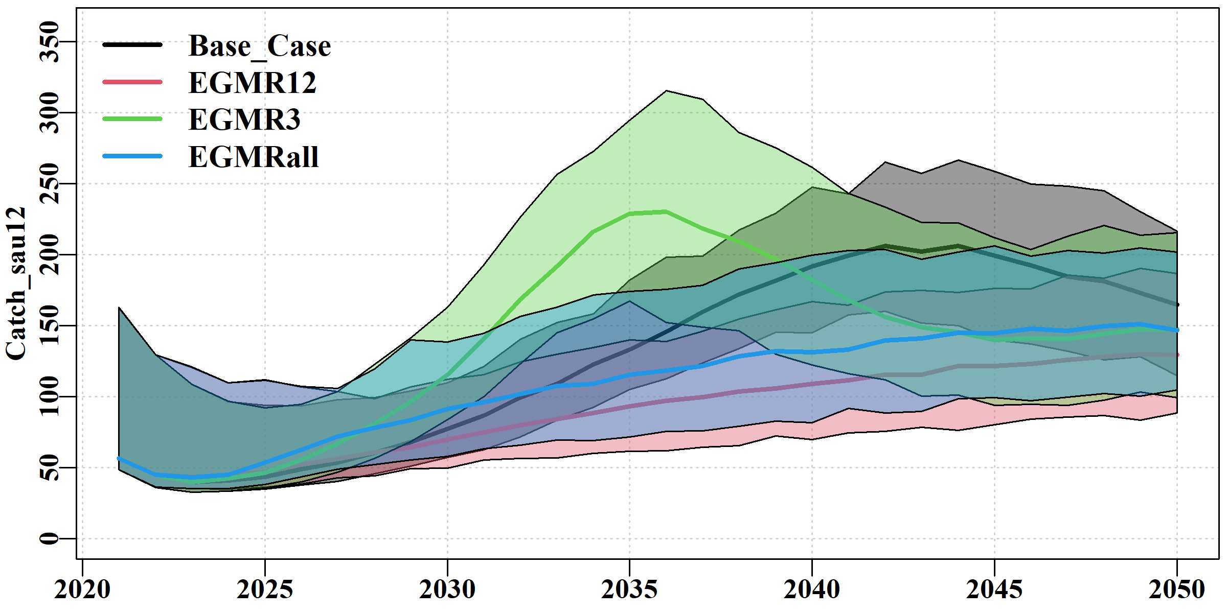
The Catches tab contains three plots and a table. The key plots are where the average annual variation of catches is plotted for each scenario x each sau, this is repeated for the sum of catches over the first five years, and then for the first 10 years. The effect on sau12 become apparent once again in each of these plots. The final table contains the boxplot statistics for each comparison and each sau.
The catchBoxPlots is similar to the catches tab but contains boxplots for each sau for each scenario, for the three harvest strategy performance measures: aavc, sum5, and sum10.
The cpueBoxPlots tab contains boxplots for each sau within each scenario of the years taken to achieve the maximum cpue, and for each sau x scenario, the years taken to achieve the median maximum cpue.
The C_vs_MSY tab contains plots for each scenario and sau of the ratio of the predicted catches divided by the predicted MSY for each sau, which is one of the preferred MSE performance measures. In the current example, the trajectory of return to near the MSY might be better illustrated by a new ribbon plot as seen in the zone tab, and this will be implemented.
The ScenarioPMs tab contains a set of histograms of the deviations from a loess fitted, in each scenario, to all replicates across years. The mean and standard deviation of those distributions are tabulated below. This is a different measure of catch variability.
The zone tab contains ribbon plot outlines of each scenario’s 90th quantile bounds for the total zone statistics, overlaid so that areas of overlap and differences become clear. The use of rgb colours allows for transparency so that the degree of overlap can become clear. When too many scenarios are included in a plot this can become confusing.
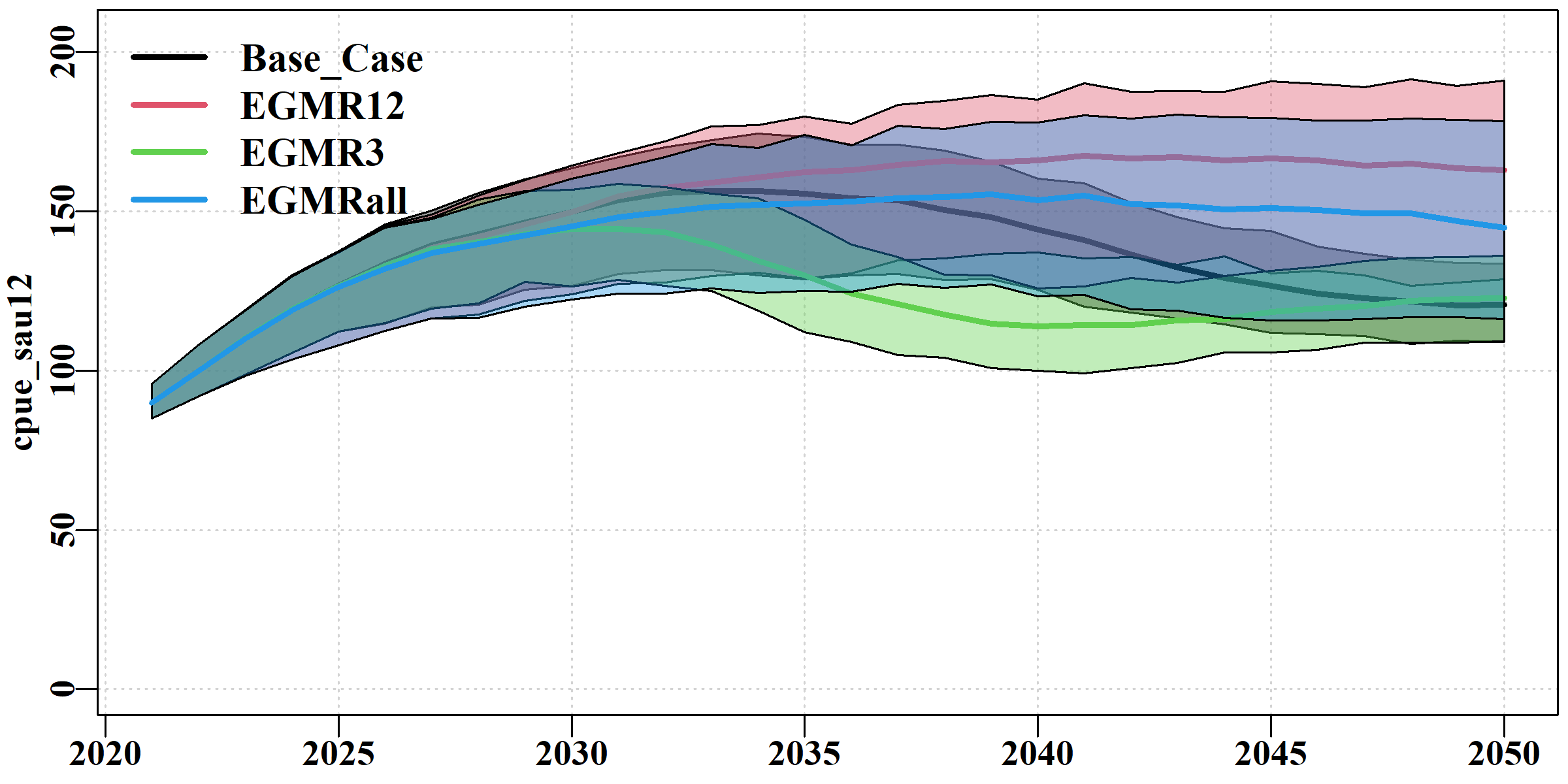
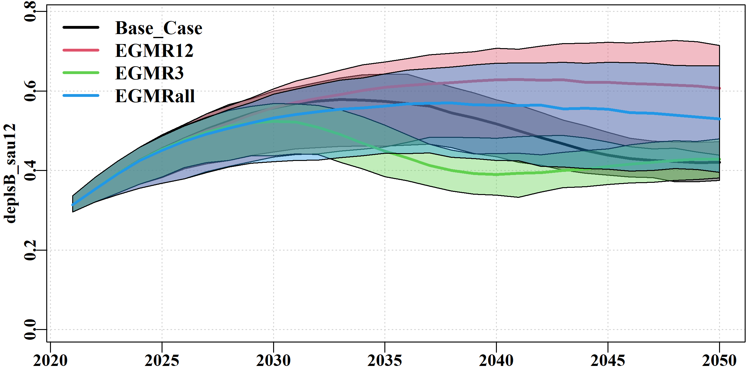
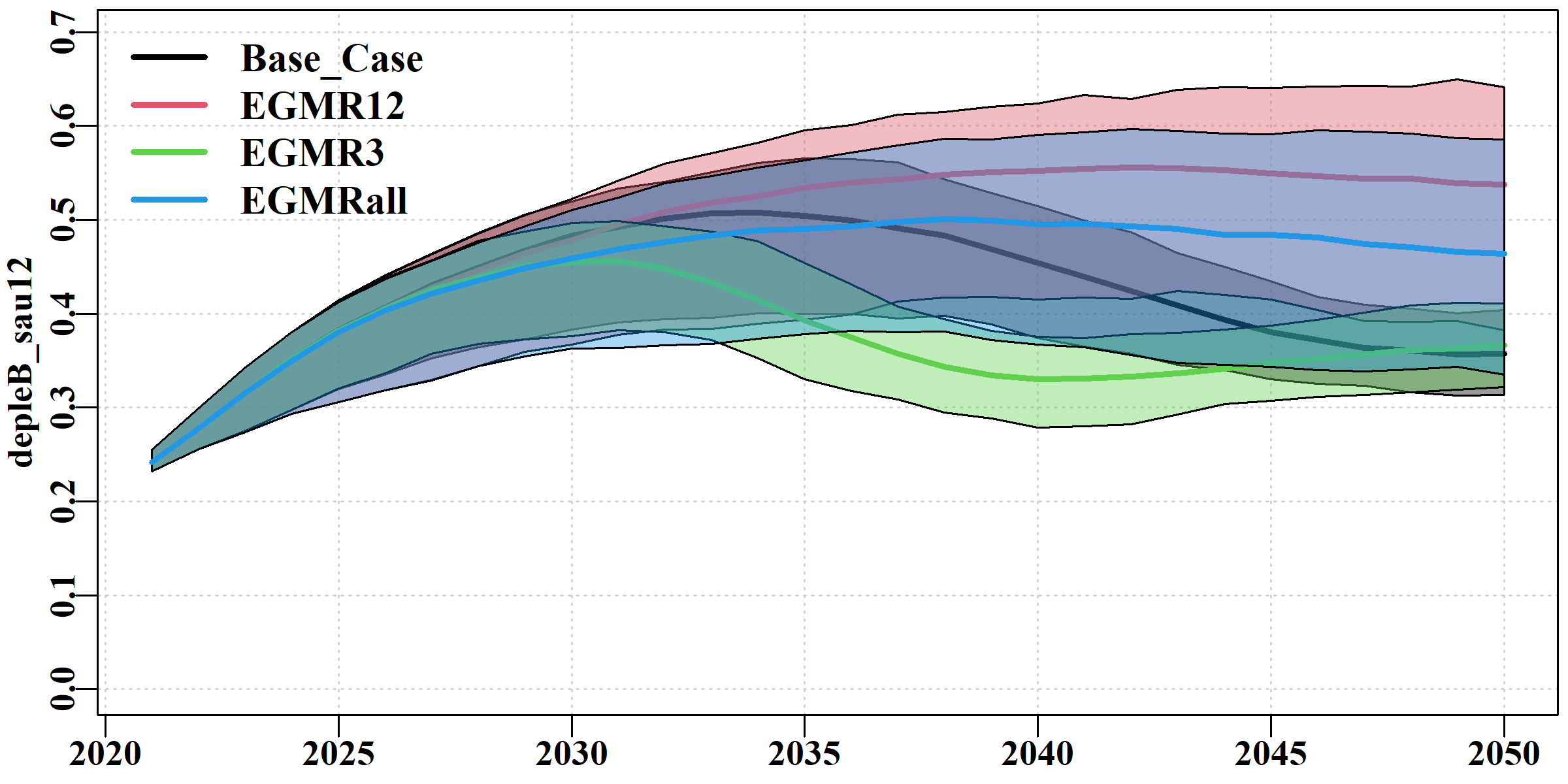
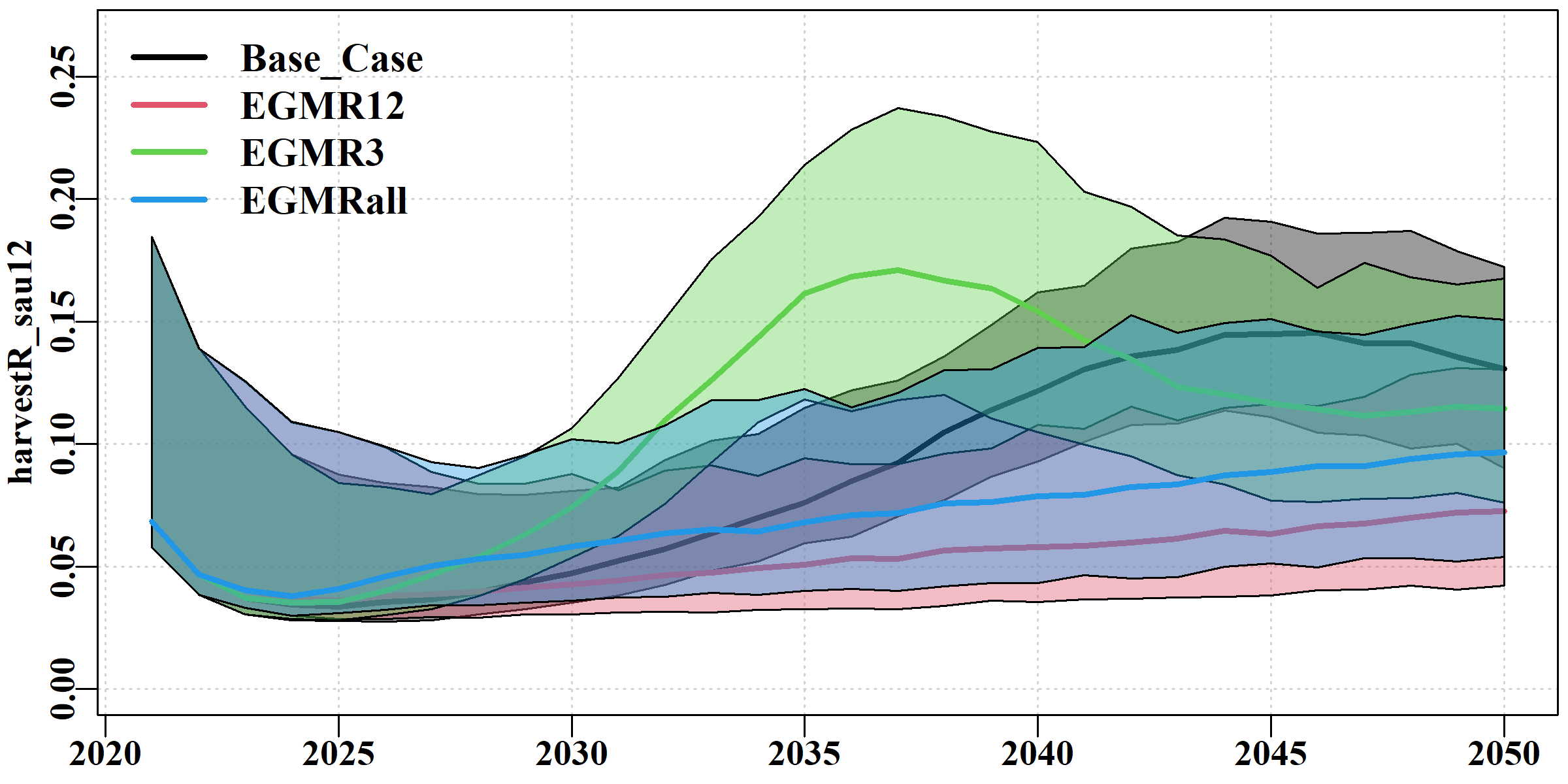
The Catch, cpue, deplsB, depleB, and the harvestR tabs all use the same ribbon plots as in the zone tab except they repeat the information in the Dynamics tab in a manner that makes comparisons simpler for some people.
The Catch tab uses ribbon plots to illustrate the overlap and differences between the scenarios in terms of the combined catch for each sau. The use of semi-transparent colours helps to discern the level of overlap.
The cpue tab uses ribbon plots to illustrate the overlap and differences between the scenarios in terms of the cpue in each sau. Once again, the use of semi-transparent colours helps to discern the level of overlap.
The deplsB tab uses ribbon plots to illustrate the overlap and differences between the scenarios in terms of the mature biomass depletion levels in each sau.
The depleB tab uses ribbon plots to illustrate the overlap and differences between the scenarios in terms of the exploitable biomass depletion levels in each sau. In the example, the differences found in sau12 become very clear. The results here are similar to those exhibited with the spawning biomass depletion, but remain of interest because the exploitable biomass is more closely associated with cpue than the spawning biomass.
The harvestR tab makes it very clear that MR3, sustains oscillatory behaviour in terms of harvest rates (and other dynamics) much longer than the other scenarios.
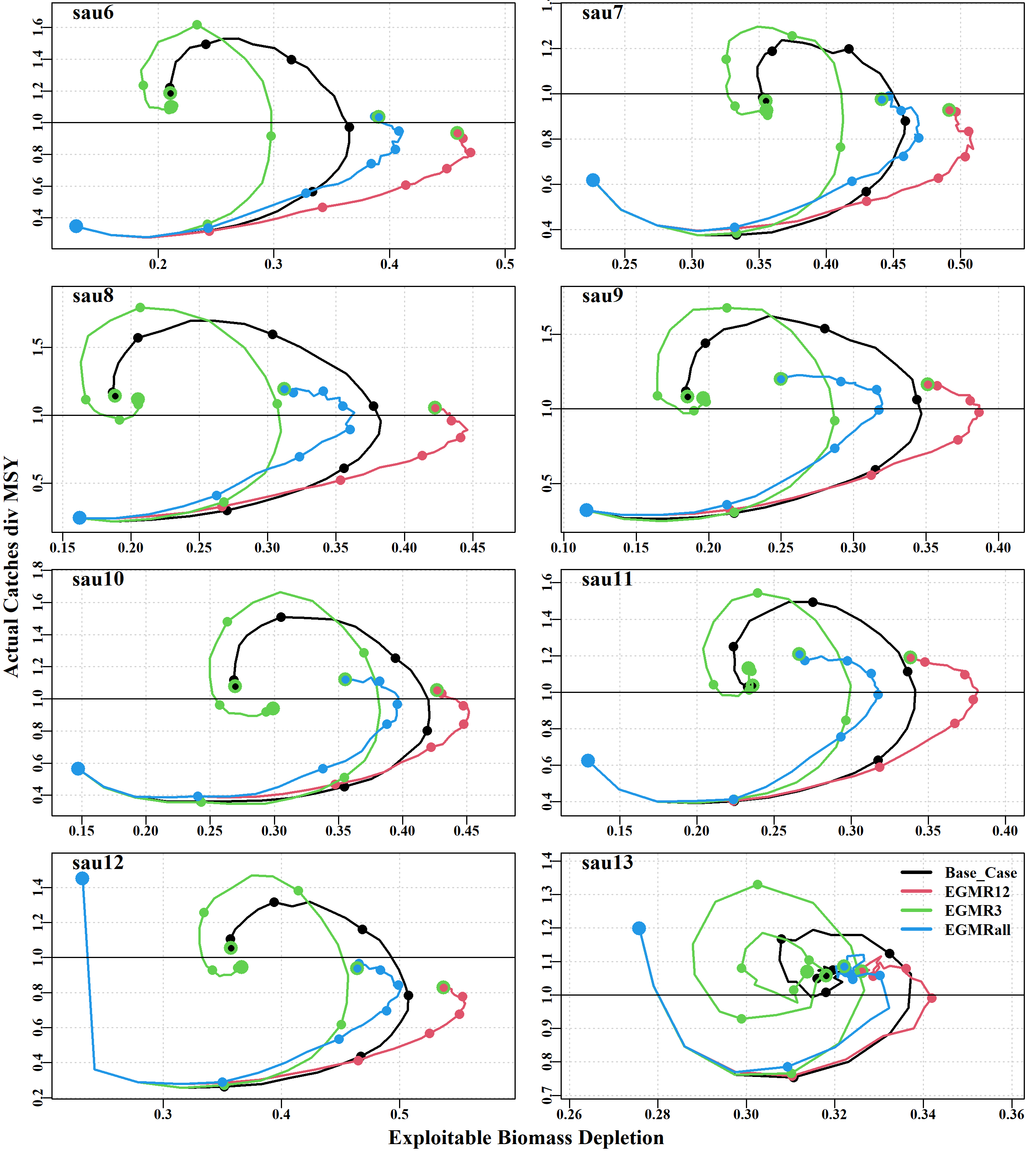
Finally, the phaseplots tab contains ten plots depicting, for each sau the effect of the different scenarios on the relationships, during the projections, of the following combinations of variable (using the medians in all cases): 1) actual catch/MSY vs exploitable biomass depletion, 2) actual catch/MSY vs mature biomass depletion, 3) actual catch/MSY vs Mature Biomass/Bmsy, 4) actual catch vs exploitable biomass depletion, 5) Actual catches vs mature biomass depletion, 6) Aspirational catch vs mature biomass, 7) Aspirational catch vs Mature Biomass depletion, 8) CPUE vs Actual catches, 9) Annual harvest rate vs actual catches, and 10) Actual catches vs Exploitable biomass.