Model Dynamics
The operating model generates the population dynamics for a simulated abalone zone by following the numbers-at-size through time of each of the component populations within each of the sau. It does this by including how each is affected by natural mortality, somatic growth, fishing mortality, and recruitment. The model developed in Haddon et al. (2013) and Haddon and Helidoniotis (2013), and further developed in Haddon & Mundy (2016), used separate vectors of numbers-at-size to describe the cryptic \(N_t^C\) and emergent \(N_t^E\) components of each population. While this can be considered as a more realistic representation of nature further testing demonstrated it was relatively inefficient. Here the model is somewhat simplified through the cryptic and emergent components of the population being contained in the single vector \(N_t\), where \(N_t\) is assumed to be the numbers-at-size (shell length in mm) at the start of each year \(t\). This simplifies the equations and helps speed the calculations although with this approach the effect of emergence needs to be included explicitly in some of the equations describing the dynamics (see the Selectivity section below).
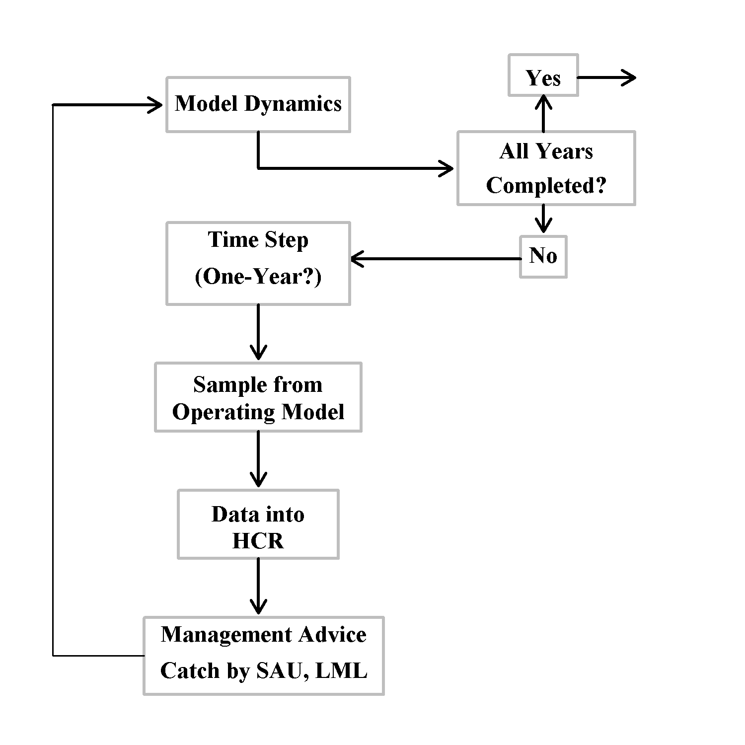
Being based upon difference equations, the model structure adopted to describe the assumed annual dynamics, begins at the start of each year and involves a number of steps: 1) half of the survivorship from natural mortality being applied first, 20 this is followed by individual growth, 3) then survivorship from fishing mortality (if fishing occurs), 4) followed by the remaining survivorship from natural mortality, 5) finally, each population \(p\), will give rise to \(R_p\) recruits in year \(t\), and if any larval dispersal occurs (described by the movement matrix Phi, \(\mathbf{\Phi}\)), would lead to the re-distribution of a small proportion of those recruits among the populations (Miller et al, 2009), and they are then added to the first size class of each population vector, \(p\), at the end of year \(t\), \(\mathbf{N_{p,t}}\), which is equivalent to be ing the start of hte following year. If natural mortality is implemented as half natural mortality, that is \(S_{h} = e^{-M_p/2}\), twice a year, with other dynamics between the natural mortality events then the dynamics for the numbers-at-size can be represented in matrix notation (which is read right to left) as:
\[
{\mathbf{{N}_{p}^{t+1}}}={\mathbf{{\Phi}R_p}}+{S}_{p}^{h}{\mathbf{A_p}}{\mathbf{G_p}}{S}_{p}^{h}{\mathbf{N_{p}^{t}}}
\tag{7.1}\]
where \(S_{p}^{h}\) is the survivorship of population \(p\) following half of the instantaneous natural mortality in each population, \(M_p\) (some small variation between populations is assumed), \(\mathbf{A_p}\) is the survivorship following the imposition of any fishing mortality occurring in population \(p\) (which is implemented as vector multiplication with the vector result of \(\mathbf{G_p}{S}_{p}^{h}\mathbf{N}_{p,t}\)), \(\mathbf{G_p}\) is the growth transition matrix for population \(p\), and \(\mathbf{{\Phi}{R_p}}\) is the vector of recruits, \(\mathbf{R_p}\), from each population multiplied by the movement matrix \(\mathbf{\Phi}\) among populations, and then added into each size-class within \(\mathbf{N_{p,t+1}}\) (the same as if it had been added at the end of the year, \(\mathbf{N_{p,t}}\); because the end of each year is the same as the start of the next.
The survivorship following the fishing mortality rate over a year is defined as the complement of an annual harvest rate A:
\[A_{p,L}=\left(1-{s_{p,L,t}H_{p,t}} \right) \tag{7.2}\]
where \(A_{p,L}\) is the survivorship of length class \(L\) for population \(p\), \(s_{p,L,t}\) is the selectivity of length class \(L\) in year \(t\), and \(H_{p,t}\) is the fully selected harvest rate in year \(t\) for population \(p\) (the harvest rate being the proportion of exploitable biomass taken as catch). We explicitly use exploitable biomass because the standard use of a legal minimum length (LML) in abalone fisheries can lead to the exploitable biomass being very different from the mature biomass.
an alternative view of the survivorship would be:
\[\mathbf{A_{p,t}}=e^{-\mathbf{s_{p,t}}F_{p,t}} \tag{7.3}\]
where \(\mathbf{s_{p,t}}\) is the vector of selectivity-at-length (or size). Strictly, selectivity is assumed to be equal for all populations within a zone (although as selectivity is combined with emergence, which varies by population, the \(p\) subscript is also required; see below), and \(F_{p,t}\) is the fully selected, instantaneous fishing mortality rate for population \(p\) in year \(t\). This simplification means that now the transition from cryptic and emergent no longer needs to be included in the annual dynamics. However, it does require that selectivity is now a combination of selectivity-by-diver and Emergence, which is only influential on the final selectivity if the logistic used to describe emergence overlaps the legal minimum length (which is quite possible in some areas of the western zone where the size at maturity can be relatively large and in the early years of the fishery in Tasmania and the LML was only 127mm).
Model Initiation
Model initiation will always begin with each population being assumed to be at equilibrium in the absence of fishing. At equilibrium, \({\mathbf{N}^{*}}\), the absence of fishing mortality implies that survivorship from the annual harvest rate equals one, \(\mathbf{A = 1.0}\), which can therefore be omitted from the initiation):
\[\mathbf{{N}_{p}^{*}}= \mathbf{{\Phi}R_p} + \mathbf{{S}_{p}^{h}}\mathbf{{G}{S}_{p}^{h}}\mathbf{{N}_{p}^{*}}\]
If it is assumed that there is no larval movement, \(\mathbf{\Phi = I}\), the Unit matrix, then that matrix can also be ignored (for the time-being) in the dynamics, which can be re-arranged to obtain an analytic expression for the equilibrium numbers-at-length \(\mathbf{N_p^*}\) (Sullivan et al, 1990):
\[{\mathbf{N}_p^{*}-{S}_{p}^{h}\mathbf{G_p}{S}_{p}^{h}\mathbf{N_p^{*}} = \mathbf{N}^{*}(\mathbf{I}-{S}_{p}^{h} \mathbf{G}{S}_{p}^{h})= \mathbf{R_p}}\]
which, finally, implies (Sullivan et al, 1990):
\[\mathbf{{N}_{p}^{*}}=\left (\mathbf{{I}-{S_{p}^{h}}}\mathbf{{G}{S}_{p}^{h}} \right )^{-1} \mathbf{{R_p}} \tag{7.4}\]
If, however, there is even a minor degree of larval dispersal, and for blacklip abalone in Tasmania a value of 0.5 percent (0.005) between populations is plausible, then the analytical solution is no longer valid. In practice, within aMSE, the R-package from this project (R Core Team, 2024; Haddon, 2024), the analytic solution is used to obtain the starting point for an iterative application of the unfished dynamics until an equilibrium is obtained (see the help for the function testequil).
Initial Depletion
By definition the model is initiated at an unfished equilibrium. However, having the complete fishery history is not a luxury afforded to every fishery so there will be instances where prior to conditioning the mdoel prior to applying the known historical catches, all or at least some SAU may already be depleted to different degrees. The level of such depletion may be suggested by the application of the sizemod size-based integrated assessment program to each SAU (see chapter on Conditioning the MSE with the sizemod Package). Alternatively, alternative levels may be applied in a hypothetical manner to determine their influence.
If an initial depletion is required this is input in the control file under the ZONE section in the initdepl vector, with a value for each SAU (even if it equals 1.0, meaning no initial depletion). This preliminary depletion is conducted within the depleteSAU() aMSE function. If the initdepl value for an SAU is < 1.0, then this uses a simple trial and error search for the harvest rate that depletes each SAU to a level closest to the value in initdepl and uses that value to deplete the populations within the SAU so the final depletion is as close as can be to the required value. Only then does the conditioning (fitting the operating model to the available observations) occur. The dynamics for applying any initial depletion level is set to use the selectivity that is reported for the first year of observational data.
Biology and Stock Related Statistics
Emergence
A logistic curve (Haddon, 2011, 2021) can be used to describe the transition from the cryptic to the emergent component of the population, but this could only become influential on the dynamics if natural mortality differs between the two components or if the emergence logistic overlaps with the selectivity curve, and or the Legal Minimum Length (LML).
\[\begin{matrix}
E_{p,L}=\frac{1}{1+exp{\left({-{log}(19)(L-L_{E_{p}50})/(L_{E_p95}-L_{E_p50})} \right)}}
\\
E_{p,L}=\frac{1}{1+exp{\left({-{log}(19)(L-L_{E_p50})/\delta_p} \right)}}
\end{matrix} \tag{7.5}\]
where \(E_{p,L}\) is the proportion of size-class \(L\) that are emergent in population \(p\), and \(L_{E_p50}\) and \(L_{E_p95}\) are the usual logistic parameters defining the lengths at which 50% and 95% are emergent in population \(p\). The term \(\delta_p\) is the constant \((L_{E_p95}-L_{E_p50})\). Emergence from crypsis only becomes an issue for the dynamics of the model if they are considered to have different natural mortality rates within crypsis and/or when the emergence curve overlaps with the selectivity curve (which it can do when the LML is low, e.g. 127mm early on in Tasmania, especially on the west coast). Where the selectivity and emergence curves overlap then the proportion remaining in crypsis would act as a refuge, effectively reducing the fishing mortality on those size classes.
Selectivity
Selectivity-by-diver is assumed to be equal across populations within a zone, but a \(p\) subscript could be added if different LML were expressed in different parts of a zone (this might be the case if different LML were imposed in different parts of the same zone, which can occur in Tasmania!). In the operating model Selectivity, \(s_{L,t}\) for length \(L\) in year \(t\) needs to be defined by year to permit changes in the LML to be reflected in the selectivity by divers. This implies that rather than a single vector of values, a matrix of selectivity values will be required, one column per year. Each year’s selectivity is defined using a lower-case \(s\) to distinguish it from Survivorship:
\[s_{L,t}=\frac{1}{1+{exp \left [ {-{log}(19)( L-{L_{s}}50)/{\delta_s}} \right ] }} \tag{7.6}\]
where \(\delta_s=L_s95-L_s50\).
Strictly, in case the emergence curve overlaps the selectivity curve, to define selectivity we should multiply the selectivity-at-length by the emergence-at-length (element x element, or Hadamard, multiplication). That way, if there is overlap it will alter the selectivity appropriately, and if there is no overlap then selectivity will not be affected. Importantly, because emergence varies by population, this means that the selectivity expressed would not necessarily be the same across all populations.
\[\begin{matrix}
s_{p,L,t}=s_{L,t} \times E_{p,L}
\\
{\mathbf{s_{p,t}}}={\mathbf{s_{t}}} \otimes {\mathbf{E_{p}}}
\end{matrix} \tag{7.7}\]
Growth
The growth from size-class \(i\) to size-class \(j\) is described by the elements of a growth transition matrix defined by:
\[
\begin{aligned}
& \begin{matrix}
{{G}_{p,i,j}}=\int\limits_{-\infty }^{{{L}_{i}}+\frac{LW}{2}}{\frac{1}{\sqrt{2\pi }{{\sigma }_{p,j}}}\exp \left( -\left[ \frac{{{L}_{i}}-{{{\bar{L}}}_{j}}}{2{{({{\sigma }_{p,j}})}^{2}}} \right] \right)}dL & {{L}_{i}}={{L}_{Min}} \\
\end{matrix} \\
& \begin{matrix}
{{G}_{p,i,j}}=\int\limits_{{L_i}-\frac{LW}{2}}^{{{L}_{i}}+\frac{LW}{2}}{\frac{1}{\sqrt{2\pi }{{\sigma }_{p,j}}}\exp \left( -\left[ \frac{{{L}_{i}}-{{{\bar{L}}}_{j}}}{2{{({{\sigma}_{p,j}})}^{2}}} \right] \right)}dL & {{L}_{Min}}<{{L}_{i}}\le {{L}_{Max}} \\
\end{matrix} \\
\end{aligned}
\tag{7.8}\]
where \(G_{p,i,j}\) is the probability of growing from size class \(j\) into size class \(i\) in population \(p\), \(LW\) is the size-class width, \(\sigma_{p,j}\) is the standard deviation of the normal curve describing the growth increments of animals starting in size class \(j\) in population \(p\), \(L_{i}\) is the length of size class \(i\), and \(\bar{L}_{j}\) is the mean growth increment of animals starting from the mean of size-class \(j\). \(L_{Min}\) and \(L_{Max}\) are the minimum and maximum size-classes, with the maximum being treated as a plus group. To ensure that all columns sum to 1.0 (to prevent growth implying losses or gains of its own), and to make \(L_{Max}\) a plus group, the final row of the matrix is modified for each column \(j\) as:
\[{{G}_{{p,L}_{Max,j}}}={{G}_{{p,L}_{Max,j}}}+\left( 1-\sum\limits_{i={{L}_{1}}}^{{{L}_{Max}}}{{{G}_{p,i,j}}} \right) \tag{7.9}\]
The expected mean growth increment from size-class \(j\) (so it grows into size class \(i\)) is defined using an inverse logistic growth curve that has been found to describe blacklip abalone growth well (Haddon et al. 2008; Helidoniotis et al., 2011):
\[{\bar{L}}_{p,i,j}={{L}_{p,j}}+\frac{Max\Delta L_p}{1+{exp \left[ {log\left( 19 \right)\left( {{L}_{p,j}}-{L_{p,j}50} \right)/\delta_{p,j}} \right ]}}+{{\varepsilon }_{{{L}_{p,j}}}}\]
\(Max \Delta L_p\) is the maximum growth increment for the population \(p\), \(L_{p,j}50\) and \(L_{p,j}95\) are the usual logistic parameters defining the initial lengths at which 50% and 5% of the maximum growth increment are expressed (\(\delta_{p,j}\) is simply the 95% minus the 50% parameters). Note that the \(log(19)\) is positive, which inverts the logistic curve (compare with the equation for emergence; Equation 7.5). The \({\varepsilon}_{{L}_{p,j}}\) is the variation around the mean expected growth increment. It is assumed to be normally distributed with a standard deviation that varies with the growth increment (Haddon et al. 2008):
\[{{\sigma }_{{{L}_{p,j}}}}=\frac{Max{{\sigma }_{L_p}}}{1+{exp \left[ {log\left( 19 \right)\left( {L_{p,j}}-{L_{p,g}95} \right)/\delta_{p,j,\sigma}} \right ]}} \tag{7.10}\]
The \(\left( L_{Max}-{{L}_{p,g}95} \right)\) remains a constant and can be parameterized as such (\(\delta_{p,g,\sigma}\)). Alternative descriptions of this variation, such as the use of a power law (Haddon, 2021), may be explored for their impact. Additional growth curve description options could be included in the R package aMSE (Haddon, 2025) if requested by users.
An important influence on the growth increment estimates is the negative bias that appears to be introduced by the tagging methods used in their estimation (See Haddon et al, 2013, page 191, Figure 70). This means that when conditioning the abalone operating model, it will be necessary to compare the predicted unfished numbers-at-size with those obtained from the fisheries catch-at-size. In that earlier work, after using the best estimates of growth increment from tagging, the predicted size-distribution of the unfished population had a smaller average size than the observed frequencies in the catches from a non-pristine fishery. Clearly modifications to the growth parameters were required and options are discussed in the growth section of the Conditioning_the_MSE chapter.
Weight-at-Length
The weight-at-length, \(W_L\), relationship involves two constants:
\[W_{p,L}=a_pL_p^{b_p} \tag{7.11}\]
During the conditioning of the model it is possible that an observed power relationship that exists between the two parameters can be used instead of estimating both (see Haddon et al, 2013, page 209, Figure 75). Using this has the advantage that any correlation between the two parameters is maintained even when random pairs are used.
Maturity-at-Length
Maturity at size, \(m_{p,L}\), uses an alternative logistic curve, again with two parameters, \(\alpha\) and \(\beta\), only this time \(L_{m_p50} = -{\alpha_p}/{\beta_p}\) and the inter-quartile distance is \(2{{log}}3 \beta_p = 2.197225 \beta_p\).
\[m_{p,L}=\frac{exp(\alpha_p + \beta_p L)}{1+exp(\alpha_{p} + \beta_p L)}=\frac{1}{1+\left(exp(\alpha_p + \beta_p L) \right)^{-1}} \tag{7.12}\]
such curves are best fitted to observed data using a Generalized Linear Model that uses binomial residual errors (see the associated R package biology).
Spawning and Exploitable Biomass
Mature or spawning biomass needs to include numbers-at-size by maturity-at-size and weight-at-size. The operating model (OM) operates at the population scale but the ‘predicted’ data from the OM needs to be at the SAU level. Hence, the outputs from each population need to be combined in a valid manner (see later under Sampling). Whatever the case for sampling, we will still need population-based estimates of such things as exploitable biomass, numbers-at-size, and so on, so methods for combining the appropriate populations into a single SAU are required. Some, such as numbers-at-size, will need simple summation while others, such as cpue, might require catch-weighted values. A population-based estimate of spawning biomass at time \(t\), \(B_{p,t}^{S}\), can be obtained through:
\[B_{p,t}^{S}=\sum\limits_{L={{L}_{Min}}}^{{{L}_{Max}}}{\left( {m_{p,L}}{W_{p,L}}{N_{p,L,t}} \right)} \tag{7.13}\]
Spawning biomass is, like exploitable biomass, calculated in the same units as the \(W_{p,L}\) equation (dependent upon what parameter values are used). If that is in grams then it requires division by 1e6 to estimate tonnes, if in kg then division by 1000 is required. Exploitable biomass, when used to calculate CPUE, is estimated after half of natural mortality and growth have occurred and before any fishing mortality occurs in any single year. Remember that the selectivity for each population, \(s_{p,L,t}\) includes any effects of Emergence:
\[B_{p,t}^{E}=\sum\limits_{L={{L}_{Min}}}^{{{L}_{Max}}}{{{s}_{p,L,t}}{{W}_{p,L}}G_{p,L,j}{e^{-M_p/2}}N_{p,L,t}} \tag{7.14}\]
where the exploitable numbers-at-size \(L\) in year \(t\), \({{N}_{p,L,t}^{E}}\), is obtained from:
\[{{N}_{p,L,t}^{E}}=G_{p,L,j}{e^{-M_p/2}}{{s}_{p,L,t}}N_{p,L,t} \tag{7.15}\]
where \(N_{p,L,t}\) is the numbers-at-size \(L\) at the start of year \(t\) for population \(p\).
For internal consistency, however, exploitable biomass is also reported as start-of-year values as well as mid-year values, and so is simply the sum across size-classes of the final numbers-at-size at the end of the previous year by the selectivity times the weight-at-length:
\[B_{p,t+1}^{E}=\sum\limits_{L={{L}_{Min}}}^{{{L}_{Max}}}{{{s}_{p,L,t}}{{W}_{p,L}}N_{p,L,t}} \tag{7.16}\]
where \(B_{p,t+1}^{E}\) is the start-of year exploitable biomass (equals the end of year exploitable biomass).
Catchability and CPUE
At least in the Tasmanian blacklip abalone fishery, the relationship between catch-rates and catches is usually observed to be linear, hence the relation between catches and effort is also linear. Because of this catch-rates are assumed to have at least some influence over the distribution of catches among areas. Observed catch-rates (cpue) would naturally be expected to be variable through time and across areas and so are modelled as:
\[I_{t,p}={q_p}\left(B_{p,t}^E\right)^{\lambda}{e^{N(0,\sigma_q)}}
\]
where \(I_{t,p}\) is the cpue in year \(t\) for area \(p\), \(q_p\) is the catchability coefficient within population \(p\). \({B_{p,t}^E}\) is the mid-year exploitable biomass in year \(t\) and area \(p\), with a non-linearity coefficient of \(\lambda\), and \({e^{N(0,\sigma_q)}}\) is a Log-Normal random deviate, with \(\sigma_p\) being the standard deviation of the catchability coefficient \(q_p\). If \(\lambda = 1.0\) then the relationship between cpue and exploitable biomass is linear, values other than \(\lambda = 1.0\) lead to non-linear relationships, which can make rather a large difference to the \(q_p\) value. Given how important the use of cpue is in all Australian abalone harvest strategies, this is one assumption whose influence is in dire need of testing. We are using \(p\) as a sub-script for population (or area of persistent production), because in the conditioning each population within each Spatial Assessment Unit corresponds to a particular area within that SAU. Effectively, area and population are the same thing in the model.
Annual Model Dynamics
Once each population is initiated its dynamics can be projected forwards a year at a time depending on how much catch is expected to be taken or how much effort is expected to be focussed into each population. The population initiation sets up the equilibrium numbers for the properties defined for each population. Then, given a specific harvest rate for each population they can be projected forward in yearly steps. This projection is based around how the numbers-at-size change through fishing, growth, natural mortality, and recruitment. As before, the fishing mortality rate over a year is defined as the complement of an annual harvest rate and is distributed down the diagonal of an otherwise zero matrix A:
\[
A_{p,L} =\left(1-{s_{p,L,t}H_{p,t}} \right)
\]
where \(A_{p,L}\) is the survivorship of length class \(L\) for population \(p\), \(s_{p,L,t}\) is the selectivity of length class \(L\) in year \(t\), and \(H_{p,t}\) is the fully selected harvest rate in year \(t\) for population \(p\) (the harvest rate being the proportion of exploitable biomass taken as catch). We can define the survivorship from applying half of natural mortality as follows:
\[
{S}_{p}^{h}=e^{-M_p/2}
\]
\({S}_{p}^{h}\) does not need to be a vector as multiplying a matrix or vector by a constant is simpler and quicker. We apply this survivorship twice in a year with the other dynamics occurring between:
\[
\mathbf{{N_{p}^{t+1}}}={{S}_{p}^{h}}\left[{\mathbf{G_p}}{\mathbf{A_{p}^{t}}}{{S}_{p}^{h}}{\mathbf{N_{p}^{t}}}\right] + {\mathbf{{\Phi}R_p}}
\]
Recruitment Processes
Recruitment is described using a vector with all new recruits allocated to the first size class and all other size classes being set to 0. This may need modification if small size classes are used (perhaps 1mm) and post-larval forms are variable in size. A Beverton-Holt stock recruitment relationship was assumed, as re-parameterized by Francis (1992), with a and b parameters that were restructured in terms of steepness, \(h\), unfished mature or spawning biomass, \(B_{0}^{S}\), and the average unfished recruitment level, \(R_0\):
\[a_p=\frac{4h_p{R_{p,0}}}{5h_p-1}\text{ and }b=\frac{{B_{p,0}}\left( 1-h_p \right)}{5h_p-1}\]
Using this re-parameterization the Beverton-Holt relationship becomes:
\[R_{p,t}=\frac{4h{R_{p,0}}{B_{p,t}^{S}}}{(1-h_p){B_{p,0}}+(5h_p-1){B_{p,t}^{S}}} e^{\varepsilon_{p,t}-\sigma_{p,R}^2/2}\]
where \(\varepsilon_{p,t}\) is defined as:
\[\varepsilon_{p,t}=N \left(0,\sigma_{p,R}^2 \right)\]
The expected residual error distribution around the recruitment is log-normal; \({\sigma}_{p,R}\) is the standard deviation of the natural logarithm of the recruitment residuals, and \(-{\sigma}_{p,R}^{2}/2\) is a bias correction term that ensures that the time series of estimated recruitment values relates to the mean rather than the median recruitment level (Hastings & Peacock 1975). This requires, for each population, that \(h_p\), \(R_{p,0}\), \(B_{p,0}\), and \(\sigma_{p,R}\) be defined for each population, and for each year that \({B_{p,t}^{S}}\) be estimated. Should deterministic recruitment be required (as when calculating the unfished, equilibrium zone structure), then set \(\sigma_{p,R}\) to a very small number (when 1e-08 is squared this is the smallest number possible on most computers with 15 significant digits).
\(A_{p,0}\) is the virgin biomass per recruit and is defined as the mature stock biomass that would develop given a constant recruitment level of 1. Thus, at a biomass of \(A_{p,0}\), distributed across a stable size distribution, the resulting recruitment level would be \(R_{p,0}=1\). \(A_{p,0}\) acts as a scaling factor in the recruitment equations by providing the link between \(R_{p,0}\) and \(B_{p,0}^{S}\). \(A_{p,0}\) can thus be estimated by setting the annual recruitment level to 1, obtaining the equilibrium size distribution using unfished dynamics. At the virgin biomass per recruit, \(A_{p,0}\), the average unfished recruitment level, \(R_{p,0}\), is related directly to the unfished mature, or spawning, biomass, \(B_{p,0}^{S}\):
\[B_{p,0}^{S}={R_{p,0}}{A_{p,0}}\]
In Tasmania, during the conditioning, the average unfished recruitment level for each SAU (AvRec = \(R_{0}\)) is adjusted so that the fit of the predicted CPUE is close to the observed CPUE for each SAU. The populations within each SAU are defined using the Tasmanian GPS logger data to identify areas of persistent productivity (see the Conditioning section). Then the \(R_0\) for each SAU is distributed among the populations in proportion to the relative yield reported for each of the GPS defined areas of persistent productivity (APPs, which we refer to as populations). Without a time-series of such detailed GPS data then the relative size of each population could be defined by randomly selecting (from a log-normal distribution) an initial unfished average recruitment, \(R_{p,0}\), which, given the equilibrium size distribution, provides an estimate of each population’s unfished mature biomass \(B_{p,0}^{S}\).
Larval Dispersal
The annual dynamics include recruitment but a small proportion of each population’s larval production can disperse away from that population. To be general we use a matrix of the potential movement from population to population but, given the linear structure to most reefs around coastlines very few cells in the matrix will be filled. The diagonal of the movement matrix defines the proportion of larvae that are expected to settle within the population that generates them. The immediate sub-diagonal and super-diagonal relate to the movement between adjacent populations. This simplification is used in the operating model because while a small amount of movement is known to occur (Miller et al, 2009), little or nothing else is known about that dispersal.
Alternative matrix structures could be generated to account for more complex spatial arrangements of populations but such things would need to acknowledge they were based on speculation rather then even approximate estimates.
\[\Phi =\begin{matrix}
{{p}_{1,1}} & {{p}_{2,1}} & 0 & 0 & 0 & 0 & 0 \\
{{p}_{1,2}} & {{p}_{2,2}} & {{p}_{3,2}} & 0 & 0 & 0 & 0 \\
0 & {{p}_{2,3}} & {{p}_{3,3}} & {{p}_{4,3}} & 0 & 0 & 0 \\
0 & 0 & {{p}_{3,4}} & {{p}_{4,4}} & {{p}_{5,4}} & 0 & 0 \\
0 & 0 & 0 & {{p}_{4,5}} & {{p}_{5,5}} & {{p}_{p6,5}} & 0 \\
0 & 0 & 0 & 0 & {{p}_{5,6}} & . & . \\
0 & 0 & 0 & 0 & 0 & . & {{p}_{n,n}} \\
\end{matrix}
\]
Fleet Dynamics
The application of any harvest control rule in this complex spatial model will entail the translation of SAU level aspirational catches (which should sum to the zone’s TAC), into catches applied to each individual population within each SAU. Of course, the aspirational catches per SAU derived from the harvest control rules (HCR) within each harvest strategy will not be taken exactly, The overall TAC will eventually constrain total catches, but some SAU will experience larger catches than expected, and others will experience smaller catches. As a result, the application of the TAC as catches to particular populations requires two steps.
The first step is to include variation into the aspirational catches for each SAU from the HCR and then scale them until their sum equals the original TAC. The second step requires that each SAU’s actual catch is distributed across their component populations in some manner that reflects plausible fleet dynamics.
The assumption is made in the Tasmanian HS that the sum of the catches across the SAU equates to the TAC. If ever the TAC were not completely caught this assumption would obviously have to change. Each year the aspirational catches for either the zone TAC or for each SAU will be determined by application of the harvest control rule for whatever harvest strategy is being used. In Tasmania, the harvest control rule uses a multi-criterion decision analysis (mcda) based around different aspects of cpue. In the operating model this is implemented initially without error.
\[C_{u,t,hcr}={C_{u,t-1}} \times multhcr\]
where \(C_{u,t-1}\) is the aspirational catch from SAU \(u\) in year \(t-1\), \(C_{u,t,hcr}\) is the aspirational catch from SAU \(u\) in year \(t\), and \(multhcr\) is the previous year’s acatch multiplier derived from whatever HCR is used. It is important to understand that it is the aspirational catches that are modified each year, not the actual catches.
The new \(TAC_t\) will be:
\[TAC_t={\sum\limits_{u=1}^{nSAU}C_{u,t,hcr}}\]
The first step on the way to setting the potential actual SAU catch is to include Log-Normal variation to the SAU exploitable biomass on the assumption that the divers gain an appreciation of how much is present in each SAU, but they make mistakes and availability varies across years so there is a misallocation of effort:
\[B_{u,t}^{E,*}={B_{u,t}^{E}}e^{\varepsilon_{u,t}-\sigma_{B}^2/2}
\]
where:
\[\varepsilon_{u,t}=N \left(0,\sigma_{B}^2 \right)\] \(\sigma_B\) is the standard deviation of the variation that occurs between the real exploitable biomass and the perceived distribution of exploitable biomass across SAU’s, which also includes other sources of uncertainty.
This variation is introduced into the potential SAU catches using:
\[C_{u,t}^*=TAC_t \times \frac{B_{u,t}^{E,*}}{\sum{B_{u,t}^{E}}}\]
where \(C_{u}^*\) is the actual SAU catch scaled to the new TAC.
A useful diagnostic for use during conditioning, and during model runs, would be to examine the predicted variation between the actual catches and aspirational catches determined by the HCR, if one has such data from a real fishery. Otherwise, it should be characterized from the outputs, which will allow its variation to be examined for plausibility.
Calculation of MSY
The maximum sustainable yield for each population is estimated for each one using a numerical approach that characterizes the expected production curve but starting with the equilibrium unfished population (or app) and sequentially applying a sequence of harvest rates for two or three times the number of historical years of data until it approximates an equilibrium yield for each applied harvest rate. The maximum yield achieved across the range of harvest rates is the MSY. The precision of such numerical methods is constrained by the steps selected between the individual harvest rates. The smaller the increments on harvest rate the finer the resolution. The dynamics of this numerical process, by default, uses the selectivity that will be applied at the end of the projection years.
If, for some, currently un-imagined, reason the selectivity from an alternative year is wanted then the index for that year (between 1 and hyrs + pyrs) can be put into the selectyr argument for the do_MSE() function.