5 The Input Files
5.1 aMSE Requirements
There are a number of requirements when conducting a Management Strategy Evaluation of alternative harvest strategies on an abalone fishery using the aMSE R package. It is currently best to use the RStudio integrated development environment, as this facilitates the installation of different R packages, and the editing and running of the R files used to conduct the actual scenario runs (see the Using the aMSE Software chapter).
The R packages required to run a scenario include at least:
- aMSE the main R package containing the operating model and auxiliary functions used.
- codeutils an R package containing numerous utility functions that are common to many simulation tasks.
- hplot an R package containing functions that facilitate the generation of various plots.
- makehtml an R package used to generate the multi-tabbed web-pages that can display the results generated. Not strictly required for running the scenarios but is helpful for displaying the results in an accessible manner.
- jurisdictionHS.R a source R file containing functions unique to a particular jurisdiction’s harvest strategy, or a package such as:
- TasHS is a new R package that encapsulates the harvest strategy used in Tasmania, which is used as an alternative to having a jurisdictionHS.R. The input constants used by some of those Tasmanian HS R functions still need to be declared in hsargs before running the MSE. Using an R package rather than an R source file helps guarantee that the same software is used in all scenarios and makes it easier to maintain or modify the harvest strategy as required. In the examples herein, a stable but cut-down version of TasHS called EGHS is used.
These five packages are available from https://www.github.com/haddonm.
- knitr an R package used in vignette preparation and the production of formal tables in aMSE’s output (obtainable from CRAN).
Most importantly, for this chapter, there are also a number of other data files required for a scenario run and these are all .csv files. In the sections below we will go through their structure and contents in detail to act as a guide to their format and functioning. Each can be generated using the template functions within aMSE (see the Using_aMSE chapter for details):
- a control_scenario.csv file (whose name can be anything the user wishes), that holds control options, many other constants, and identifies other input files.
- a saudata.csv file, that holds parameterizations of the biological properties of the sau and the populations that make up the operating model.
There may also be other data files if such data are available, these include:
- a size-composition of commercial catch data file (default from the rewritecompdata() function is lf_WZ90-20.csv, which is also used in the control file from ctrlfiletemplate())
- a size-composition of fishery-independent survey file, with the same internal format as the fishery size-composition file.
When using the R package aMSE a typical scenario run would entail a number of fundamental steps, although most of these are not immediately obvious tpothe user:
- Initiate each population within each sau in the operating model with its biological properties.
- Generate the equilibrium unfished zone across all populations and estimate the productivity of each population (and hence each sau and the total zone).
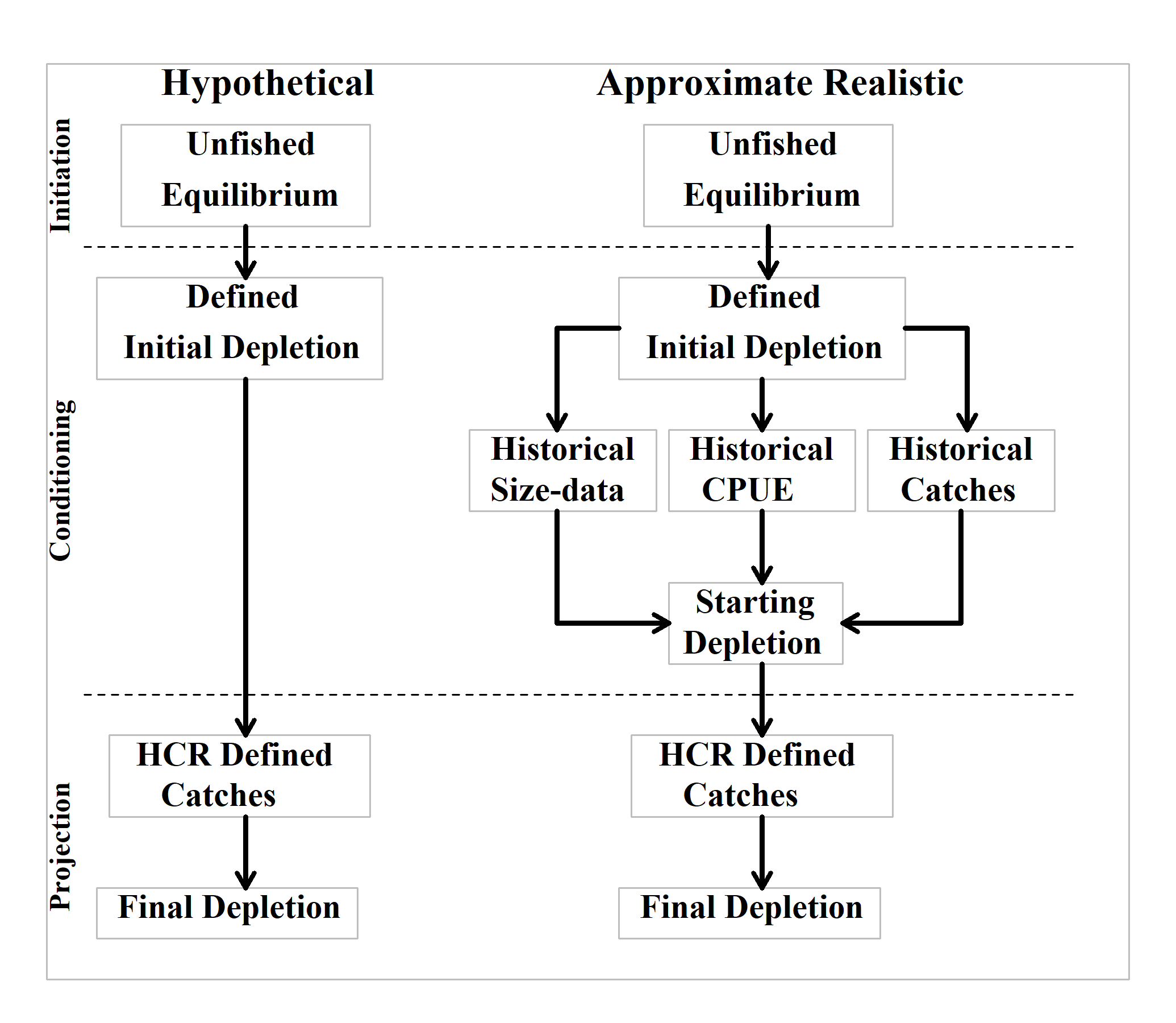
- Condition the operating model using either a hypothetical depletion or apply historical fishery data until the simulated zone is ready to be projected under control of the particular harvest strategy being considered (Figure 5.1).
- Conduct the projections and summarize the results.
5.2 File Locations for each Scenario
Within aMSE, for each scenario considered, it is designed so that all related input files (control, data, and size composition data, (and jurisdictionHS.R if that is being used rather than an HS package), and all result files will be contained in the same directory. Within the aMSE code, this directory is referred to as the rundir (as in run-directory). It is suggested that each scenario run be given a unique name that is then used as the rundir name (the postfixdir as described in the Using aMSE chapter). For example, if examining the influence of the legal minimum length (LML) on the outcome of using a particular harvest strategy (perhaps using the TasHS R package) one might have the following scenarios: rundir = “EGlml140”, “EGlml145”, “EGlml150”, and so on, all contained in a sub-directory named ‘scenarios’ (or whatever you wish; for example, Malcolm, is a good name, though you may be able to think of more appropriate ones). This would facilitate future comparisons by simplifying identification and selection of those scenarios to be compared. The names also suggest they are all variants of the “EG” basecase scenario. But of course, a user may name their rundir whatever they wish. The aim of aMSE is to facilitate running an MSE on abalone, not to force people to work effectively or efficiently!
The intent is that the control.csv, saudata.csv and the lf_data.csv files (and jurisdictionHS.R file if you have one) are stored in the rundir for each given scenario explored. This may entail duplicating the saudata.csv, lf_data.csv, and jurisdictionHS.R files between scenarios (one reason an HS R package is a sensible option) so care needs to be taken that if one changes these underlying files then those changed files need to be propagated across all sub-directories in which they are used. This is the responsibility of the operator. A simple way of making such copies has been illustrated when discussing the comparison of scenarios in the Comparing Scenarios chapter.
Here we will focus solely on the control and data files. There are functions to generate data file templates for each of the data-file types ctrlfiletemplate(), datafiletemplate(), and rewritecompdata(), which uses the internal data set data(lf). These can be run and the resulting templates edited to form the required files, this also automatically illustrates the required format. Alternatively, another option is to use the example data-files, made available with the aMSE package, which can be saved, copied and edited appropriately.
Similarly, within aMSE, there are functions to read in each type of data-file. If there is a formatting error within the data-file it should throw an error which identifies where it has gone wrong. Further development is intended to these error checks. Using the template functions and editing the results can be simpler than starting from scratch.
The input data-files, currently, are all required to be .csv files where components with multiple values use a comma as a separator. This makes their preparation using software such as Microsoft Excel relatively simple. They can also be edited directly in the editor pane of RStudio (or any other text editor).
The first of the two files is the control_scenario.csv (I name mine by including reference to the scenario, as in controlM15h7L75.csv, (natural mortality M=0.15, steepness h=0.7, and lambda L=0.75). This file contains a wide range of settings concerning the structure of the Operating Model as well as where to find any historical conditioning data from a given fishery (catches, cpue, recruitment deviates), if such conditioning is required. The second file would then be named saudataM15h7L75.csv and contains the data that is used to define the biological properties of each sau that make up the simulated zone. The rest of this document provides a detailed description of the contents and format of these files. The third file, another data file, would contain the size-composition data used to condition the scenario, if available.
If the user has used longer filenames to describe their scenarios this can lead to many plots becoming confused as the scenario names are used in the figure legends when making comparisons. This is why do_comparisons() has an altscenes argument, that allows alternative scenario names to be allocated for use in the figures.
5.3 The Conditioning Requirements
There is a spectrum to the degree to which the operating model needs to be conditioned on a real fishery. At the least specific, one still has to include a spatial structure that would reflect a typical abalone stock. In aMSE the top level is the zone, which can contain even a single SAU, which must contain one or more populations. Hence the smallest simulated zone would constitute a single SAU with a single population (this might be used to compare the effect of included an array of populations within an sau). The example data-sets within aMSE exhibit a spatial structure of 8 SAU with a total of 56 populations. This hierarchy can be customized to suit a particular jurisdiction and species, and one could then include what might be deemed typical characteristics of growth, maturity, emergence, and other details, including variation among the different populations found within each SAU. Even with such details it would remain a generic abalone MSE (Figure 5.1).
It is possible to take such conditioning a step further and customize the details of the biology of each SAU, or even each population making up the spatial structure, to reflect the biology known for a real fishery zone (assuming there are field data available). One could also scale predicted productivity and cpue to match a real fishery. This would be less generic but still not exactly fitted to a real fishery. The detailed spatial structure internal to the operating model is what makes it impossible to fit the operating model to fishery data as a whole. However, it might still be possible to fit the productivity and fishing history of individual SAU to real fishery data and thereby gain estimates of actual productivity and possibly even recruitment deviates (see Using_sizemod_to_Condition the SAU). Of course, while this latter approach would appear, at first glance, to be the best strategy for examining a harvest strategy, as it might operate in a real situation, it is also the most demanding in terms of data and difficulty. One can spend large amounts of time iteratively improving an operating model fit to observed catches, length-composition, and CPUE data for each SAU (Figure 5.1). While this is a fine way to spend time (a lot of time, and I really mean a lot of time) it is also a good strategy to remember that there is a spectrum of how closely one needs to reflect nature and that some questions about harvest strategies do not require the best possible fit to a real fishery to remain useful for determining the implications of alternative management options (see for example, Pourtois et al, 2022).
5.4 The control_scenario.csv File
The control file is a .CSV file made up of a series of sections and each will be described in turn. The values expressed in this document may differ from those generated by the ctrlfiletemplate() function, but the descriptions are valid. Within the control.csv file (which can have any name you wish, it does not have to be control.csv, though it does have to be a .csv file), the main section headings are usually written using capital letters for increased clarity. The correct spelling of such section title is important, as is the spelling of the variable names in the first column. The order of the sections does not need to be strictly maintained but the order of any components within each section must be maintained as described. This is required because in a number of cases they are being parsed in sequence, though many are also being obtained explicitly by name (which is why typing/spelling the names correctly is also important; the template files are all correct). Where the labels or names are not clear as to the intent of the variable then a description can be given to the right of the actual values. Comments can be inserted anywhere outside of any of the sections. This is all exemplified in the .csv file generated by ctrlfiletemplate(), which we will assume was given the default name controlEG.csv.
To aid understanding this document it would help the reader to have a copy of the .csv file generated by ctrlfiletemple() open in a window.
5.4.1 DESCRIPTION
At the top of the controlEG.csv file is an optional description section that can be used to describe the objective of the scenario implied by the control and population files. The author can add as many lines of text to this section as desired as, currently, it is not used in the model run. This may change later so it may act as meta-data for each run. It would be useful to treat this section as such meta-data anyway.
DESCRIPTION
Control file containing details of a particular run
Modify the contents to suit your own situation
I have added these next lines, which do not influence reading the file
If you wish you should modify the contents of this description to suit
the scenario being executed, use as many lines as required for
your own description.
5.4.2 START
The start section currently has four components, a name for the particular run (which gets used on the home tab/page of the output web-page but is most useful when comparing scenarios so make it informative!), the full name of the saudataEG.csv file (which is expected to be found in the same rundir as the controlfile). In each case, note the use of commas to separate a variable’s label from each variable’s value (cannot be seen if opened in Excel, but as long as the file is saved as a csv file all will be well). The hopefully descriptive text after each variable’s value(s) is ignored by the program and can be expanded if desired (as long as it remains as a single line, the comments below are expanded to include more explanation but you should not have multiple lines). Such descriptive text should not include commas as this will break it up into separate Excel cells
START
- runlabel, Base_Case, label for particular scenario. Very important when comparing scenarios.
- datafile, saudataBC.csv, name of saudata file = saudataBC.csv
- bysau, 1, 1=TRUE, 0 = FALSE are we expecting data by SAU or population. Generally, one would use by sau, but an option exists to operate with populations explicitly. (see Conditioning by Population.).
- parfile, NA, name of file containing optimum parameters from sizemod, this is used to simplify transferring information from sizemod to aMSE during conditioning. Generally, this is NA, which means it gets ignored (see the chapter on Using sizemod to condition the SAU).
5.4.3 zoneCOAST
The zoneCOAST section (an odd/old name, which may change to become something more descriptive, but once something is named then coding inertia can set in) currently contains four components.
zoneCOAST
- replicates, 100, number of replicates normally at least 250 or 500, in the code this is found in glb named reps.
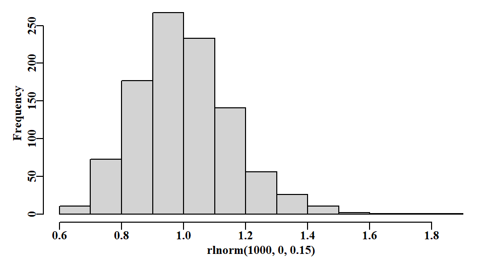
- withsigR, 0.35, recruitment variability eg 0.35, this literally varies recruitment in a Log-Normal fashion during projections and the last few years of the conditioning.
- withsigB, 0.1, process error on exploitable biomass. This affects the fleet dynamics so that, in Tasmania, the actual SAU catches end up rather different from the aspirational catches, though they all sum to the TAC. Elsewhere it could be used in the equivalent fleet dynamics function within the JurisdictionHS.R source file or R package.
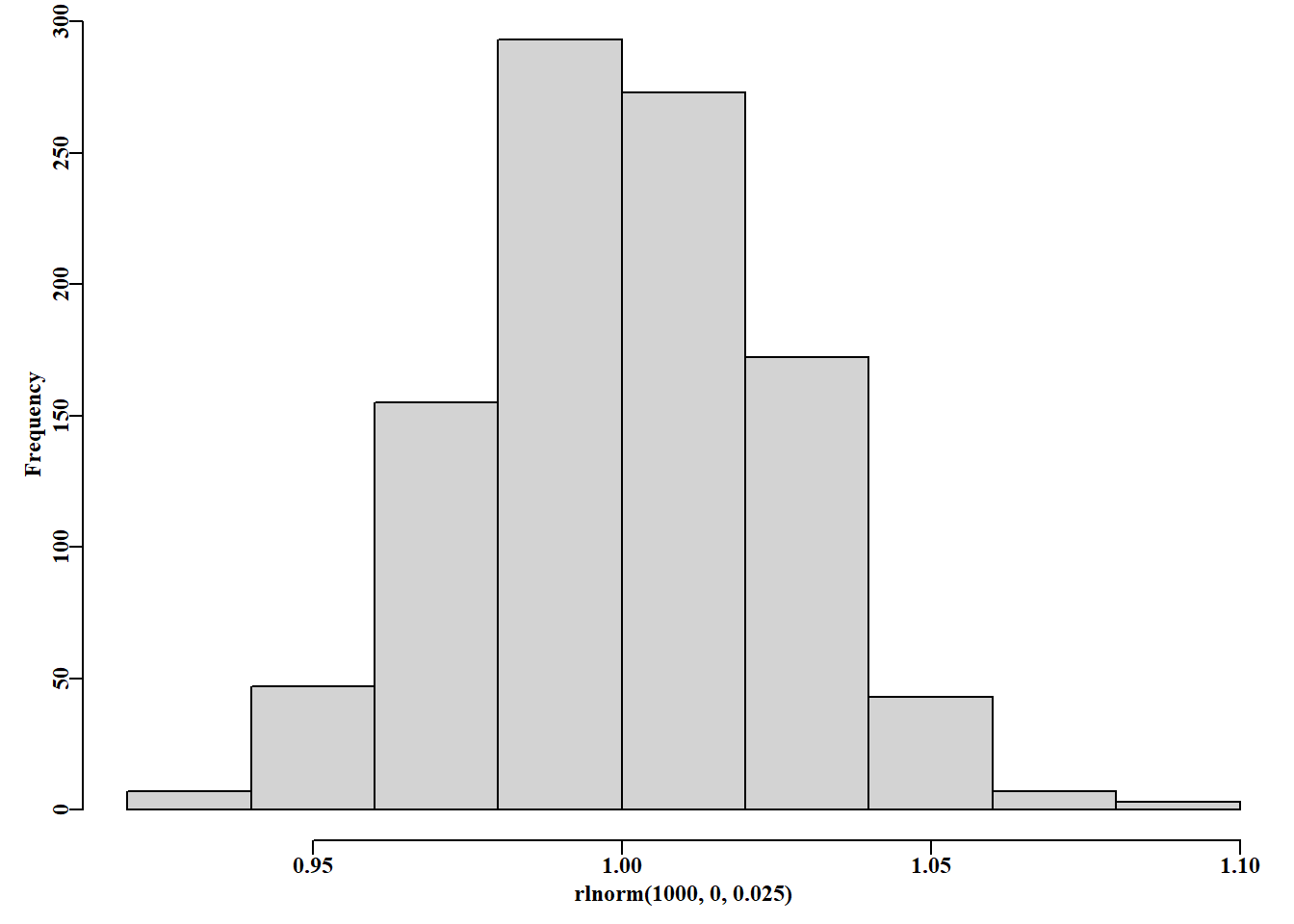
- withsigCE, 0.1, process error on cpue calculations. This will vary the relationship between cpue and exploitable biomass by including Log-Normal errors. For example, a value of 0.025 will varying the apparent exploitable biomass in individual model events between 0.9 - 1.1 times the actual value.
In the code base, the three sources of variation (withXXXX) reside in the ctrl object.
withsigR relates to the year-to-year recruitment variability. This does not include any special recruitment events or recruitment deviates that may be included. During the generation of the equilibrium, unfished model, recruitment variation is set to a very small number, 1e-08, so that recruitment processes are effectively deterministic off the Beverton-Holt stock recruitment relationship. While there appears to be no evidence of auto-correlated recruitment residuals the intent is that these will eventually be included as an option (see Operating Model Structure for further details of the model equations). It is possible to include exceptional events in particular years within the projections that influence recruitment and/or survivorship. This is intended to allow for the exploration of the implications of such things as marine heat waves, exceptional storms, and other potentially damaging events. Details are given in the Perturbations within Projections chapter.
\[R_{p,t}=\frac{4h{R_0}{B_{p,t}^{S}}}{(1-h){B_0}+(5h-1){B_{p,t}^{S}}} e^{\varepsilon_{p,t}-\sigma_{R}^2/2}\]
where \(\varepsilon_{p,t}\) is defined as:
\[\varepsilon_{p,t}=N \left(0,\sigma_{R}^2 \right)\]
withsigB the fleet dynamics of where divers elect to take their catches within an SAU mean that the actual catches from each SAU differ from the aspirational catches allocated to each SAU according to whatever harvest control rule is used. This will be determined within each jurisdictions HS R package, and may be different to the description given here, which only reflects the case in Tasmania. This is implemented by first allocating catches to the SAU in a deterministic manner and then modifying them by imputing variability to the perceived distribution of biomass among SAU, denoted \(u\), which is then propagated across component populations:
\[B_{u,t}^{E,*}={B_{u,t}^{E}}e^{\varepsilon_{u,t}-\sigma_{B}^2/2}\]
where:
\[\varepsilon_{u,t}=N \left(0,\sigma_{B}^2 \right)\]
\(\sigma_B\), withsigB, is the standard deviation of the variation that occurs between the real exploitable biomass and the perceived distribution of exploitable biomass across SAU’s, and also includes other sources of uncertainty.
This variation is introduced into the potential SAU catches using:
\[C_{u,t}^*=TAC_t \times \frac{B_{u,t}^{E,*}}{\sum{B_{u,t}^{E}}}\]
where \(TAC_t\) is the sum of the HCR’s aspirational catches in each year \(t\). One diagnostic used during conditioning (see the DiagProj tab in the webpage) is to examine the variation between the actual catches and the aspirational catches previously determined by the HCR, if one has such data. Otherwise, it should be characterized from the outputs, which will allow its variation to be examined for plausibility.
withsigCE designates the imprecision in the relationship between cpue and exploitable biomass. Essentially, it is used to generate a Log-Normally distributed random number about the value 1.0, which is then used to multiply the actual exploitable biomass. This is all conducted at the population scale (see oneyearcat code in dynamics.R). Given:
\[\varepsilon_{u,t}=N \left(0,\sigma_{ce}^2 \right)\]
then bias-corrected Log-Normal errors depicted as:
\[err=e^{\varepsilon_{u,t}-\sigma_{ce}^2/2}\]
If \(\sigma_{ce}\) is set extremely small (say, 1e-08), then \(err\) is essentially equal to one, otherwise some variation around 1 will occur and be introduced into the estimate of cpue or each population. This would be whether hyperstability is also implemented in the cpue.
\[CE_p=q_p \times \hat{B}_p^E \times err \times 1000\]
where \(\hat{B}_p^E\) is the average of the mid-year and end of year exploitable biomass. A \(\sigma_{ce} = 0.025\) value of provides a range of multipliers on the exploitable biomass of between 0.9 and 1.0:
5.4.4 ZONE
Again, the use of commas to separate variable values is essential. The zone is defined in terms of the number of SAU (spatial assessment units) it is made up of.
ZONE
- nSAU, 8, number of spatial assessment units eg 2
- SAUpop, 3, 3, 5, 7, 9, 9, 12, 8, number of populations per SAU in sequence. The phrase, ‘in sequence’ relates to the idea of distributing the SAU, and their contained populations, along the coastline in an approximately linear manner. This simplifies the larval dispersal matrix, which currently assumes the populations are aligned along the coastline approximately linearly.
- SAUnames, sau6, sau7, sau8, sau9, sau10, sau11, sau12, sau13, labels for each SAU
- initdepl, 1.0, 1.0, 1.0, 1.0, 1.0, 1.0, 1.0, 1.0, initial depletion levels for each SAU.
In the code, nSAU, SAUpop, and SAUnames all reside in the glb object, inexplicably, SAUnames in the glb object is called saunames. The initdepl values are held in the condC object used when conditioning the zone.
The example file from ctrlfiletemplate() inserts the number of populations among SAU that reflect the current selection in the Tasmanian Western Zone, but each simulated zone would be expected to be different. The SAUnames should only be mixtures of letters and numbers but must not contain spaces. The initdepl is the intended initial depletion before either the model run or further conditioning. If any of the initdepl values for any SAU is < 1.0 then, once the equilibrium zone is achieved it will undergo a depletion event (see the help on the function depleteSAU())
5.4.5 SIZE
The size structure range used in the example data files was originally selected to suit the Tasmanian blacklip abalone fishery. Hence it extends the midpoints of each 2mm size class from 2mm - 210mm, with the 210mm class being a plus group. These values will not necessarily make sense for other jurisdictions or species. Haliotis roie, for example, will require a much smaller upper size, and might possibly use 1mm size classes, depending on how data are collected.
SIZE
- minc, 2, centre of minimum size class, classes are 1-3,3-5,5-7…, centered at 2,4,6,…
- cw, 2, class width mm
- Nclass, 105, number of size classes, leading to a maximum midpoint of 210mm
These values lead to the dynamics being described within vectors and matrices ranging from 2 – 210 in 2mm size classes. Of course, each of these values can/should be altered to suit the biology of the species concerned. The derived midpts defining the size-classes, and the Nclass reside in the glb object.
5.4.6 RECRUIT
Larval movement between Tasmanian blacklip populations has been demonstrated to be remarkably low. Nevertheless, there will undoubtedly be some small amount of larval drift between populations, which operate on a smaller scale than the SAU within which they are found. With no generic estimates of this movement rate it is assumed that the populations are generally aligned linearly along the coastline and such larval movement is a small constant rate.
A linear arrangement along the coast is obviously an approximation but one should attempt to arrange the SAU and component populations in this manner or else the movement matrix will need to become rather more complex (which remains a possibility, but in the absence of data one can only wish you luck).
RECRUIT
larvdisp, 0.01, rate of larval dispersal eg 0.01 = 0.5 percent of recruits in each direction
The value of larvdisp is used to construct a simple larval movement matrix that assumes movement only occurs between adjacent populations at a rate of half the larvdisp value. While a value of 0.01 may appear almost trivial this does affect the equilibrium dynamics, but the effects are generally only minor. However, by including this it is now possible to determine the explicit effect of different levels of larval movement, and this would enable the importance of the relative isolation of the different species to be explored. The movement matrix is contained with the ‘globals’ object glb, where it can be tabulated and visualized.
5.4.7 RANDOM
There will often be a need to control the generation of random numbers used during both the definition of the populations and the projections. The use of a random seed is especially important when conditioning the operating model as many random numbers are used during that process and if the conditioning is intended to simulate a specific fishery, then the distribution of productivity needs to remain the same during each model run. The truth of this will become more apparent during the description of the saudataEG.csv file contents and uses in sections below.
The use of specific random seeds might be wanted, for example, if one wanted to be sure to repeat a particular analysis exactly, of perhaps to see only the effect of changing an argument, perhaps the LML, while making no other changes. So, to ensure the production of the same sequence of pseudo-random numbers, one uses set.seed. Under RANDOM we have two values, the first, randomseed is used for repeatability of population generation when conditioning the model. By default one would expect this to have a value. The second value, randomseedP is used for repeatability during the projections. Each scenario could have a different randomseed and, optionally, randomseedP, although one should think carefully about what one is comparing between scenarios when making this choice. Using the same seed for all scenarios compared ensures any differences seen are due the changes to the harvest strategy and are not due to the biological properties used. Ideally, one would conduct comparisons with the same initial randomseed. But would use both the same or different randomseedP for the projections so as to capture the fill range of variation. One can (should) use getseed() from codeutils to generate such seeds. It is recommended that one not try to generate one by oneself. The literature suggests that 12345 tends to be used more often than would be expected at random(!) so it, and others akin to it are just not good enough.
If one does not want to set the random seeds and just use any old random sequence that comes along then set randomseed and randomseedP to 0. By default, randomseedP is set to zero.
RANDOM, Set these to zero for non-repeatable starting points.
- randomseed, 3543304, for repeatability of population definitions if >0
- randomseedP, 0, for repeatability of projections by simply continuing with the sequence started by the randomseed value, if a different randomseedP is used, then a new set sequence of pseudo-random numbers will occur, or if set to NA a random new sequence will occur each scenario run.,
5.4.8 initLML
However the model is to be run (Figure 5.1), all scenarios begin by generating an unfished, equilibrium model. This includes a characterization of the equilibrium productivity of each population and this will require a description of selectivity to be used, hence we need an initial LML. The fishery productivity is altered when the LML is changed because it alters the balance between natural mortality, growth, and fishing mortality. Smaller LML do not always generate the highest levels of productivity (this becomes a yield-per-recruit problem, although that also, of course, depends upon the biological properties of growth).
initLML, 140, used to generate unfished zone if no historical catches and LML present
If the conditioning is to include the application of historical catches the different SAU may still require an initial depletion (which can be set at 1.0) and an initial LML. If conditioning on historical catches, then it makes sense to initiate the model at the LML in use at the start of the historical catches. If a generic MSE is being conducted, for example, a generic west coast Tasmania starting projections in 2020 or 2021, then perhaps initiate the model at an LML of 140, although, as in the file generated by ctrlfiletemplate(), project the dynamics forward from 2020 with an LML of 145 (see PROJLML later).
5.4.9 PROJECT
Basic information about the projection period of the simulations. Elsewhere we add together the projection years (here pyrs=30) and the historical years, hyrs, value (see CATCHES) to obtain the total number of years of the final projections. These values are found in the glb object, along with the year names for each sequence of years (as in hyrnames and pyrnames).
PROJECT, 30, number of projection years for each simulation
5.4.10 ENVIRON
The entries under the ENVIRON heading are designed to allow the introduction of exceptional events into specific years during the projections. For example, the incidence of marine heat wave events is increasing and are of such a degree that their impacts can influence subsequent recruitment and the survivorship of settled animals. If one wants to introduce such an event in a given year, or years, then define how many years after the ENVIRON header. Here we will introduce values that relate to two years of events, happening in the fifth and eighth projection years. In each case, the proportion of recruits in that year that survive is listed for each sau. Because there are two years the software expects two rows (beginning with ‘proprec’). If only one year, then there would be only one ‘proprec’ line (and so on). Following those lines are the survivorships of the settled animals, in this case, 99 percent are given as surviving, so the effect is primarily through the recruitment. Note that setting ENVIRON to zero means any environmentally induced effects are set to NULL and will have no effect. For more details and examples, see the Perturbation within Projections chapter.
ENVIRON, 0, in how many years will an event occur, 0 means have no events
eyr, 5, 8, which projection years will have an event
proprec1, 0.3, 0.3, 0.3, 0.3, 0.3, 0.3, 0.3, 0.3, one for each sau
proprec2, 0.3, 0.3, 0.3, 0.3, 0.3, 0.3, 0.3, 0.3, one for each sau
propNt1, 0.99, 0.99, 0.99, 0.99, 0.99, 0.99, 0.99, 0.99,
propNt2, 0.99, 0.99, 0.99, 0.99, 0.99, 0.99, 0.99, 0.99,
The passage of any ENVIRON objects through aMSE follows a simple path:
In inputfiles.R readctrlfile -> envimpact -> glb ->
In projection.R doprojections ->
In dynamics.R envimpact is used by both [oneyearcat & oneyearsauC]
The eyr determines which years have an impact.
If the year is in the eyr vector, then:
- in sauyearsauC, sigR is reduced by a factor of 10 and the value of the stock recruitment curve is multiplied by proprec, thus reducing the basline recruitment.
- in oneyearcat, the input numbers-at-size for that year is multiplied by the proportion surviving the environmental effect: inNt=(inN[,popn] * survP).
5.4.11 PROJLML
Under the PROJECT heading we read in a line for each of the projection years. Assuming that PROJECT > 0, then readctrlfile() looks for the heading PROJLML. The LML used in the projections are listed here explicitly so that changes through time can be easily implemented. There needs to be at least as many defined as the value of PROJECT (which becomes pyrs, see str1(glb)), here that is 30. The projLML are used to define the selectivity for each of the pyrs during the projections. Tasmania introduced a west coast LML = 150 in 2024 so that change should be included in future projections, though obviously it has been omitted from simulations made before 2024. The LML for the projections are included in the projC object.
PROJLML, need at least the same number as there are projection years
2020,145, the year and the Legal Minimum Length (LML, MLL, MLS) e.g. 140
2021,145,
2022,145,
2023,145,
…
…
2050,145,
5.4.12 CATCHES
If CATCHES is > 0 then one would need to include that number of years of historical catches by SAU along with the year and LML that was used when the catches were taken. An example is given below of the required format. If CATCHES = 0, then any data here will be ignored. If CATCHES > 0 then readctrlfile() looks for a heading CondYears and then reads in CATCHES rows with the following format. Here the catches are in tonnes.
CATCHES,58, if > 1 then how many years in the histLML
CondYears,LML,6,7,8,9,10,11,12,13, column names for convenience only
1963,127,0,0,0,0,0,0,0,0,, a line of zeros for initial equilibrium state
1964,127,1,1,1,4,3,5,4,1, the year, the LML, the catches by SAU
1965,127,2,3,4,17,15,21,19,5,
…
…
1987,132,31,84,44,251,82,339,195,64,
…
…
2019,140,16,53,5,65,81,179,251,53,
2020,145,7,27,6,39,58,129,227,50,
5.4.13 CEYRS
CEYRS is similar to CATCHES in that it defines how many years of cpue data will be read in. The required format is given below for CEYRS = 29.
IMPORTANT: If CEYRS = 0, then any cpue data will be ignored. Note that in the early years there appears to be cpue data missing from SAU6 and SAU13, which are present in the latest years. This is because, in Tasmania, zonation was only introduced in 2000, so cross-zone blocks such as 6 and 13 cannot be included prior to 2000.
,6,7,8,9,10,11,12,13, again, not used here just as labels
CEYRS,29, if >0 then number reflects number of historical CPUE records by SAU
1992, ,113.4, 94.2, 97.0, 99.4, 98.1, 100.19, ,
1993, ,116.8, 110.38, 109.37, 99.1, 107.88, 102.20, ,
…
…
2018, 106.68, 143.57, 148.43, 133.70, 104.38, 95.01, 106.88, 104.08,
2019, 92.22, 112.70, 107.11, 93.65, 91.89, 86.94, 90.03, 90.78,
2020, 92.01, 113.01, 112.10, 99.10, 92.10, 87.10, 93.10, 92.10,
5.4.14 SIZECOMP
Size-composition data is akin to the biological properties data in being potentially a large amount of data which might confuse the structure and editing of of the control file. Hence we use this to refer to a filename containing the required data. If SIZECOMP = 0 then no file will be read in, otherwise a list of filenames will be expected and these should be stored in the rundir. The filenames should begin in the row immediately below SIZECOMP.
SIZECOMP,1
lf_90-20.csv
The format of the size-composition .CSV data file should be the following, of course the years and size classes used should reflect your own data (see the output of writecompdata() for the full format):
length, sau, 1984, 1985, 1986, … , 2019, 2020
120, 7, 0,0,0, … , 0,0
122, 7, 0,0,0, … , 0,0
124, 7, 1,1,2, … , 0,0
126, 7, 1,3,4, … , 0,0
128, 7, 3,19,26, … 0,0
…, 7,
…, 7,
208, 7, 0,0,0, … , 0,0
210, 7, 0,0,0, … , 0,0
By using this format it is possible to use the function getLFdata() to read the data into the program. Try ?getLFdata. These data are read in and returned to the program within the condC object.
5.4.15 RECDEV
Conditioning the data on historical catches and cpue will entail searching for an AvRec value that approximates the long-term productivity of the unfished stock. This should place the predicted cpue approximately through the observed cpue. However, one can expect to see deviations, some relatively large. After fitting numerous example models it becomes clear that average recruitment off the stock recruitment curve provides an inadequate description of the dynamics of any abalone fishery. It is possible to adjust the rise and fall of the predicted cpue by imposing recruitment deviates in particular years. Recruitment deviates are expected to take the form of Log-Normal variation, which vary around the value 1.0. If the model predicted recruitment matched the Beverton-Holt predicted recruitment exactly this would imply a recruitment deviate value = 1.0 as each average recruitment value is multiplied by the deviate. Thus, if recruitment is taken to be lower than the stock-recruitment curve would predict, then the deviate would be less than 1.0 and if recruitment was greater than expected the deviate would be greater than 1.0. These are best fitted iniitally using the sizemod R package but if this fails through, for example, inadequate contrast in available data, then cruder alternatives exist within aMSE (see Conditioning the Operating Model).
IMPORTANT: By relying primarily on recruitment deviates to match the observed against the predicted cpue, and the observed vs the predicted size-composition data, we would be ignoring any extra non-fishing related mortality, such as marine heat-wave events or other environmentally driven mortality events. But as a first approximation it should be able to move each SAU closer to the observed state.
The format of the recruitment deviates is as follows:
RECDEV, 58
CondYears, 6,7,8,9,10,11,12,13 This line is here for convenience
1963, -1, -1, -1, -1, -1, -1 -1, -1, The -1 values mean ignore recruitment deviates
1964, -1, -1, -1, -1, -1, -1 -1, -1, The -1 values mean ignore recruitment deviates
1965, -1, -1, -1, -1, -1, -1 -1, -1, The -1 values mean ignore recruitment deviates
1966, -1, -1, -1, -1, -1, -1 -1, -1, The -1 values mean ignore recruitment deviates
…
…
1980,1.207,1.097,0.939,1.014,0.643,0.911,0.504,1.197, some SAU +ve some -ve
1981,1.083,0.140,0.500,1.547,0.591,0.503,0.066,0.645,
1982,0.922,0.915,1.130,0.994,0.790,0.995,0.807,1.067,
1983,1.019,0.933,1.129,1.114,0.887,0.923,0.784,1.360,
…
…
If a line, after the year value is >0 then values for the whole line MUST be given, even if they are merely set at 1, which implies the recruitment level should be taken off the mean of the stock recruitment relationship.
The values illustrated were derived from simple code that first searches for an optimum AvRec value, and then searches, sequentially through each SAU, for an optimum set of recruitment deviates between a given range of years. One needs to account for the expected time-lag in years between when a cohort might settle and when it then will begin to enter the fishery. The values included in the ctrlfiletemplate() function were obtained using sizemod to fit each sau’s data to an array of parameters, including recruitment deviates.
5.5 The saudataEG.csv File
This file is identified in the START section of the control file. Like the control file the saudataEG.csv file can also start off with some optional descriptive text lines.
SAU definitions listing Probability density function parameters for each variable
These are randomly allocated to each population except for the proportion of recruitment, which is literally allocated down in the popREC section
As many of these descriptive lines as required can be included. The start of input that is used by the MSE is signaled by the SPATIAL heading (remember use capital letters for the section headings where indicated and getting the spelling correct are important). The saudataEG.csv file contents are read in by the function readsaudatafile(), and each variable is identified and selected by its name (so type carefully or use the datafiletemplate() function to make a start). Despite this approach, reading the values is still split into groups that relate to their function. First there are lines describing the implied geographical spatial structure being simulated, then comes a matrix of properties for each SAU, following on from the PDFs heading.
Not all the input variables are used to define probability density functions. Thus, each of the nsau, saupop, saunames are defined explicitly after deciding on the geographical structure to impose. They need to be listed in the order in which they are expected to occur along the coast. Each population is a member of a given SAU, and here we are using the Tasmanian block number as the SAU index (and the saunames). Each SAU can have a different number of populations. These three SPATIAL inputs appear to be duplicates of those in the controlEG.csv, and they are, but are used for different purposes.
SPATIAL
nsau, 8, number of spatial management units eg 6 or in TAS’s case 8
saupop, 3, 3, 5, 7, 9, 9, 12, 8, number of populations per SAU in sequence
saunames, 6, 7, 8, 9, 10, 11, 12, 13, labels for each SAU; not used
5.5.1 PDFs
PDFs, 32,
This line is read in to determine the number of variable values to be read (the rows to the matrix). The number of columns of the matrix are defined by the nsau defined above.
The precision with which this matrix is filled will constitute a large part of any conditioning. Approximate and plausible values will produce a generic MSE whereas, tuning the matrix to the biological properties of a particular zone, and especially particular SAU, as best one can, will generate a much more specific MSE, especially if that is followed up by conditioning the resulting modelled stock on historical fishery data. Thus, if one then included historical catches and other fishery data the result would be as realistic a modelled representation as one could get when using such a complex spatial structure and without an enormous amount of data (which no-one has).
Here we only imply a plausible and generic zone, as can be inferred by the repeated values (which will still lead to different values between populations because variability is included as each population is generated - variables prefixed s, are all large enough to influence a random number). If specific values for a given population are wanted then set the respective variation value to 1e-08. All variables are sampled from a Normal distribution except for the average unfished recruitment, which strongly defines the upper productivity of each population, and is sampled from a log-normal distribution (see the function definepops()).
5.5.2 Growth
The parameters of the Inverse Logistic model describing growth (Haddon et al, 2008; Haddon & Mundy, 2016). Alternative growth functions will be implemented in the future, if desired, and will be selected in this section. In each case there is the main parameter (MaxDL, L50, L50inc, and SigMAx) followed immediately by the variation to be attributed to a given population’s value (obtained through sampling from a normal distribution). If exact or specific values are wanted for the populations in a given SAU, then set the respective variation value to 0. Estimates of MaxDL and L95 (L50inc = L95 - L50) can be obtained for a given sau by using sizemod.
DLMax ,26, 30, 30, 34, 34, 34, 34, 29, maximum growth increment
sDLMax ,2, 2, 2, 2, 2, 2, 2, 2, variation of MaxDL within each SAU
L50 ,135.276, 135.276, 135.276, …, …, …, …, …, Length at 50% MaxDL
sL50 ,2, 2, 2, 2, 2, 2, 2, 2, variation of L50
L50inc ,39, 39, 39, 39, 39, 39, 39, 39, L95 - L50 = delta =L50inc
sL50inc ,1.5, 1.5, 1.25, 1.25, 1.25, 1.25, 1.25, 1.25, variation of L50inc
SigMax ,3.3784, 3.3784, 3.3784, …, …, …, …, …, max var around growth
sSigMax ,0.1, 0.1, 0.1, 0.1, 0.1, 0.1, 0.1, 0.1, var of SigMax
5.5.3 LML
It is not impossible that different SAU operate under different LML, this allows for the generation of the equilibrium zone to reflect such variation if present. If, however, historical catches are available and are used, they are defined along with the LML used in each year and those LML are used in the zone definition instead. The entry here is only for situations where no historic data are used, but it still needs to be present under all circumstances.
LML ,127, 127, 127, 127, 127, 127, 127, 127, Initial legal minimum length
5.5.4 Weight-at-Size
The weight-at-size relationships for each population are defined using the standard equation:
\[W_{p,L}=a_pL_{p}^{b_p}\] which defines the weight of animals in population \(p\) at length \(L\). For this we need both the \(a_p\) and \(b_p\) parameters.
It was found in Haddon et al (2013; see pages 208-209) that there was a power relationship between the \(b_p\) parameter and its corresponding \(a_p\) parameter. This was useful but lacked any intuitive sense. An examination of weight-at-size relationships within sau (see the appendix on _weight-at-size vs_location) found that within sau these relationships mainly had very similar values for the ‘a’ parameter with minor variation in the ‘b’ parameter. While that variation was low, it nevertheless led to important differences between populations. So low variation is included in the exponent, ‘b’ but only extremely low variation included for the ‘a’ parameter.
Wtb ,3.161963, 3.161963, 3.161963, …, …, …, …, …, weight-at-length exponent
sWtb ,0.000148, 0.000148, 0.000148, …, …, …, …, var of Wtb
Wta ,6.4224e-05,5.62e-05, …, …, …, …, …, …, power curve intercept
sWta ,1e-08, 1e-08, …, …, …, …, …, …, variation of Wta
5.5.5 Natural Mortality
This is a troublesome variable. Previous work has generally assumed a natural mortality rate of about 0.2, but this suggests that most animals would be close to senile by the age of 23 (only 1 percent would be expected to survive that long). However, very many very large animals have been found, despite their growth characteristics implying that to reach such sizes would take much longer than 23 years (given the very slow growth rates of large animals). This casts doubt on the notion of M = 0.2, which, if traced, stems from some rather limited, and potentially flawed (blocking respiratory pores with tags) tagging data from decades ago. As with the growth characteristics, tagging may negatively affect survivorship, this potentially affecting any early tagging study of natural mortality (biasing it high). Here we have selected 0.15 as the mean or base-case against which to compare the rest, but the uncertainty means that it would be worthwhile comparing the outcomes of any HS when M = c(0.1, 0.125, 0.15, 0.175, and possibly even 0.2).
Me ,0.15, 0.15, 0.15, 0.15, 0.15, 0.15, 0.15, 0.15, Nat Mort
sMe ,0.005, 0.005, 0.005, 0.005, …, …, …, …, var of Me
5.5.6 Recruitment
The average unfished recruitment is a major influence on the productivity of each SAU and population. During conditioning it is recommended that this be one of the first variables to adjust to set-up each population’s unfished production. At very least it should be possible to determine the relative long-term production of each SAU, and this can be used as a guide to determine the relative productivity of each SAU, which should then be distributed among its constituent populations. If a time-series of GPS data-logger information is available (or potentially a series of surveys) this can be used to scale the relative productivity of each constituent population within each SAU (this is done in the propREC section of the saudataEG.csv file, as described below). The AvRec unfished recruitment (\(R0\)) value, in each case, is in linear-space for ease of use, but is commonly expressed as log(AvRec) in the model. This is defined using steepness as shown in the equations within the zoneCOAST section above. Estimates of AvRec for each sau can be obtained by using sizemod.
AvRec,217500,410000,185000,905000,760000,1440000,1350000,355000,
sAvRec,0.0001, 0.0001, 0.0001, 0.0001, 0.0001, 0.0001, 0.0001, 0.0001, R0 variation
defsteep ,0.7, 0.7, 0.7, 0.7, 0.7, 0.7, 0.7, 0.7, Beverton-Holt steepness
sdefsteep ,0.0125, 0.0125, 0.0125, 0.0125, …, …, …, ….,
5.5.7 Emergence
Emergence has been studied in Tasmania through an examination of the growth of encrusting animals and algae on the animal’s shells. The cover by algae (even encrusting algae) being taken as evidence of emergence (exposure to light). This only becomes influential if the emergence curve overlaps with the selectivity curve, which may happen when the LML is low. If no emergence data is present, then just set values so that the emergence curve always runs at smaller sizes than the selectivity curves (see later). These values below are mostly invented (for now; from very limited data) but would influence availability when the LML was down at 127mm.
L50C ,126.4222, 126.4222, 126.4222, …, … , length at 50% emergent
sL50C ,0.5, 0.5, 0.5, 0.5, 0.5, 0.5, 0.5, 0.5,
deltaC ,10, 10, 10, 10, 10, 10, 10, 10, length at 95% - 50% emergent
sdeltaC ,0.1, 0.1, 0.1, 0.1, 0.1, 0.1, 0.1, 0.1,
5.5.8 CPUE
Earlier versions of aMSE, assumed linearity between cpue and exploitable biomass and a maximum cpue was used to designate or scale the predicted cpue to match nominal observed cpue levels. Now, however, the option (the very much preferred option) is to assume hyper-stability of cpue (a non-linear relationship between cpue and exploitable biomass) and this has made the next two parameters redundant. They are retained however, as the maximum cpue that would be obtained in an unfished population can be stored in this variable once it is calculated. The values contained in this variable are no longer used but nsau values are required in each row in all cases. The variation can be set to zero (again, no longer used).
MaxCEpars, 0.4,0.425,0.45,0.475,0.45,0.45,0.375,0.3, max cpue t-hr
sMaxCEpars, 0, 0, 0, 0, 0, 0, 0, 0,
5.5.9 Selectivity
Even though there is an LML, the precision with which abalone are taken with respect to the LML is not always perfect with some legal sized animals being left behind and occasionally some just sub-legal being taken (though these observations may be due to measuring error). Here we use a simple addition to the selectivity ogive used for each population. The selL95p parameter can be estimated within sizemod, and often has values between 4 - 6. The selectivity curves used in the modelling (which are a combination of selectivity and availability) are illustrated in the Fishery tab of the MSE output.
selL50p ,0 ,0, 0, 0, 0, 0, 0, 0, L50 of selectivity, 0 = no bias
selL95p ,5, 5, 5, 5, 5, 5, 5, 5, L95 of selectivity
5.5.10 Size-at-Maturity
It was found in Haddon et al (2013; see pages 210-211) that there were relationships between the two parameters used to define the logistic maturity-at-size relationships for different populations. A fixed parameter value of -16 for the \(a_p\) parameter led to a range of plausible values for the \(b_p\) parameter. A better alternative is to use size-at-maturity data from each sau if it is available. If available it can be analysed using the biology package (the values included in the file created by the datafiletemplate() function derive from maturity samples analysed in that way.
SaMa, -22.3,-22.3,-22.2,-22.1,-24.0,-15.2,-21.2,-22.1, maturity logistic a par
L50Mat, 98.8,98.8,116.3,116.7,122.9, 112.2,121.1,105.8, L50 for maturity b = -1/L50
sL50Mat, 3, 3, 3, 3, 3, 3, 3, 3,
5.5.11 cpue Hyper-stability parameter
The lambda parameter in the equation
\[I_y=qest \times B_E^\lambda\] can define a linear relationship between cpue and exploitable biomass only when lambda or \(\lambda\) has a value of 1.0. If \(\lambda < 1.0\), then that relationship curves down to generate hyper-stable cpue values. Hyper-stability of, at least Tasmanian blacklip abalone, has now been demonstrated using the GPS logger data, and so now, in Tasmania, the base-case being used assumes a \(\lambda = 0.75\). No variation is currently included in that parameter. The qest parameter (estimated within sizemod, although it could be approximated by trial and error) is designed to scale the exploitable biomass (raised to the exponent \(\lambda\)) so that the resulting cpue matches the observed nominal scale. If \(\lambda = 0.5\) this would be equivalent to using the square-root of the exploitable biomass, which is obviously a smaller number than the original, hence the scaling factor qest needs to adjust for that appropriately for each SAU.
lambda, 0.75,0.75,0.75,0.75,0.75,0.75,0.75,0.75 ,
qest, 4.75, 2.25, 5.17, 1.63, 1.27, 0.77, 0.61, 1.45,
5.6 propREC
The propREC section provides details of the distribution of the recruitment levels across the populations within each SAU. The three columns of values are the SAU, the population index, and its expected proportion of its respective SAU recruitment each year. These values need to be set manually during the conditioning and can be varied until the dynamics approximate the desired dynamics. In Tasmania, once again the GPS logger data were able to be used to identify within each sau, areas of persistent productivity, which were equated to the populations. These varied in area and in average yield, but provided a more objective way to define the population structure within each sau than simply ascribing different numbers of populations and proportions of recruitment.
SAU,pop,propR
6, 1, 0.742, in SAU 6 about 1/6 of recruitment goes to pop 1
6, 2, 0.094, in SAU 6 most recruitment goes to pop2
6, 3, 0.163, in SAU 6 almost no recruitment goes to pop3
7, 4, 0.203, in SAU 7 a more even distribution of recruitment occurs
7, 5, 0.59
7, 6, 0.207
8, 7, 0.041
…
…
12, 48, 0.03
13, 49, 0.121
13, 50, 0.084
13, 51, 0.124, in SAU 13 there are 8 populations with variable levels
13, 52, 0.164
13, 53, 0.215
13, 54, 0.126
13, 55, 0.062
13, 56, 0.104
That completes the current structures and formats of the control.csv, saudata.csv, and size-composition data files.