3 Using aMSE
3.1 A Worked Example
Rather than continue with theoretical considerations we will begin working through an example MSE run in some detail. In this way users will see what actions are needed in practice rather than deal with more abstract notions. During the development of the aMSE R package for FRDC 2019-118, the Tasmanian western zone was conditioned on both biological and fisheries data to provide for further development and testing of the software. The summary data required are now included as default settings in the ctrlfiletemplate() and datafiletemplate() functions. In addition, we can also use the data(lfs) internal data-set and the function rewritecompdata() to generate the size-composition data required.
In this chapter, we will use these functions to produce a working example scenario that will provide an overview of what is needed to use the software and what to expect to come out of it when run. It is recommended that the help for each function and data-set mentioned in this documentation be read for a fuller understanding of what is going on. For example, after running library(aMSE), typing ?rewritecompdata, or whatever function name is of interest, into the RStudio console - see the chapter A Non-Introduction to R in Haddon (2021) for details about examining R code within a package. To read a list of all visible functions within a loaded package, in the console type ?codeutils (or whichever package is of interest). Its help screen should open. Scroll to the bottom and click on the ‘Index’ within [Package codeutils version 0.0.16 Index] and a listing of each function and its title will appear. An alternative approach is to use ls(“package:aMSE”) or ls.str(“package:aMSE”). The latter also provides the syntax of each function.
3.1.1 Requirements to Run aMSE
Before running the example, it is, of course, necessary to install the required R packages containing the software used. The following description will continue under the assumption that the user will be using R with RStudio (see https://posit.co/). If some other development environment is being used, then it will be assumed that the user will be able to adapt the following to their own system.
It is necessary to install the following R packages (and their dependencies).
The first two can be downloaded from CRAN in the usual way. In RStudio, use the Packages tab and click on Install, then type their names in the input box with a space between each one:
- rmarkdown required for the vignettes within aMSE.
- knitr required for the vignettes and for the kable function that is used in the output .html files to generate readable tables.
Four packages specific to aMSE are required for all jurisdictions (aMSE, codeutils, hplot, and makehtml). The first R package, aMSE is one of the outputs from FRDC project 2019-118, codeutils and hplot are earlier packages that now contain extra functions added during the execution of 2019-118. makehtml was developed for other uses and is simply used by aMSE to generate the internal websites that display the results. In addition, a fifth user-supplied package (or R-source file) is needed, which contains functions implementing the Harvest Strategy for the jurisdiction of interest (see the JurisdictionHS_Requirements chapter), here we will use the EGHS package. The four aMSE related R packages are available through either installation or cloning from the GitHub account at https://www.github.com/haddonm, or they can be installed from the build source files (ending in tar.gz) located in the directory: dropbox/National_abalone_MSE/aMSE_files. Obviously, the EGHS package is only required if the user is intending to use or explore the Tasmanian harvest strategy.
- aMSE is the primary package for running the MSE, it contains the functions and some data-sets that drive the MSE code-base.
- codeutils is a package containing (surprise) an array of utility functions used especially when reading files, parsing text, and so on.
- hplot is a package containing functions written in base R to assist with plotting various types of specialized graphics that aMSE uses.
- makehtml is a package used to automatically generate the HTML and CSS files that make up the summary internal web-page for displaying the many results from single scenarios using the MSE and, similarly, when comparing scenarios.
If installing from the R source files one would need to have copies of the latest version of aMSE and dependent packages sourced using the GitHub link above (where the version number is at least that shown or larger, which would imply more recent):
- aMSE_0.3.5.tar.gz,
- codeutils_0.0.15.tar.gz,
- hplot_0.0.19.tar.gz,
- makehtml_0.1.2.tar.gz, and, if using the Tasmanian HS,
- EGHS_0.1.15.tar.gz.
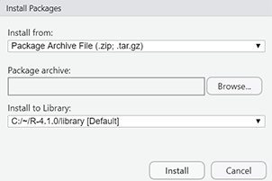
In RStudio, under the Packages tab one first presses the Install button and then uses the install from option box that pops up (each users library location will likely differ):
3.2 Running aMSE
3.2.1 Organize Scenario Results
The number of possible scenarios it is possible to generate in a relatively short time is very large so to facilitate making comparisons as simple as possible, it is best to be organized about how to save the results for each scenario. The sub-directory name and path for all the input files and the results that follow for a given scenario is named in the code as the rundir (for hopefully obvious reasons). For example, in the text below we will introduce what will be termed the ‘EG’ sub-directory (EG as in example). So, the rundir would be the generic path leading to all the scenario sub-directories combined with EG/, the actual scenario in this case. The scenario name EG/ is known as the postfixdir, while the generic path to all scenario sub-directories is the prefixdir. On the computer in which this example is being developed the prefixdir is, in fact, pathtopath(getDBdir(),“A_CodeUse/aMSEUse/scenarios/”) (note that the R / sub-divider can, as usual, be replaced by the double backslash, \\, if that is preferred; the getDBdir() function finds the path to the DropBox directory, to use a different prefixdir then define it however you wish). The pathtopath() function combines the character strings irrespective of what sub-divider is used or what each component starts with or ends with; In each case the sub-dividers should not be mixed as in / with \\.
Graphically, this can all be represented, as an example, so that the prefixdir would be:
..DropBox/A_CodeR/aMSEGuide/runs
and sub-directories below the ‘runs’ sub-directory might be:
- runs/EG
- runs/EGM12
- runs/EGM3
- runs/EGMall
- ..
which indicates four sub-directories where EG is the example basecase where none of the meta-rules are used. The meta-rules are used to modify the outcome of the analysis of the three fishery performance measures to more closely match the desired HS objectives. In the EGHS there are currently three meta-rules, each described later when comaprisons between HS will be made. The EGM12 is where only meta-rules 1 and 2 are used, similarly EGM3 and EGMall are where meta-rule 3 only is used and all meta-rules are used, respectively. In all cases natural mortality = 0.15, steepness = 0.7, and the hyperstability lambda = 0.75 (see the chapters on conditioning the operating model to make sense of those parameters. These four scenarios can then be compared to determine which had the most effects that best matched the desired objectives of the harvest strategy. When dealing with Windows machines a useful shortcut is to realize the classical “~” used by Unix and Linux systems, refers to the user’s “Documents” directory. Thus, on my own computer, in R, path.expand(“~”) gives rise to “C:/Users/Malco/Documents” (partly because Windows 11 is pathetic and its default user directory cannot spell Malcolm). Of course, this being Microsoft, one cannot rename either the default ‘user’ or the ‘Documents’ directories but it can be used if required.
3.2.2 A Possible Workflow
Once the R packages are installed then a potential workflow might begin with these nine steps (see the R code chunks below in Section 3.3 for code details):
- For each scenario to be considered, select or create a directory somewhere in your own system that will become the rundir within which the control file and the data files are placed (and all the results will be written as separate files). The directory path pointing to the different scenarios, each in their own rundir, is termed the prefixdir, which in the example to follow will be C:/Users/Malco/Dropbox/A_CodeR/aMSEGuide/runs/, but obviously a user will need to set up their own directory structure. One then identifies a postfixdir, which is appended to the prefixdir to form each rundir, so, initially, here we will have a postfixdir = EG/. If one then uses the function confirmdir(), it either confirms that the rundir exists or it asks whether you would want to create it, after which it creates that sub-directory ready for your work. Again, read the function’s help for more options, and/or use ?confirmdir. If the ‘ask’ argument is set FALSE then it will just create a missing directory without asking, so check the spelling of your postfixdir first if you use that confirmdir() option.
In the text below (section 3.3) there are example R-code blocks which can also be found in the associated file. You will find such a directory, called EG, in the Dropbox/National_abalone_MSE/aMSE_files/scenarios directory. You could copy that to the location of your choice. In it you will also see a file called run_aMSE.R, which contains the code as described across the code blocks below. Once the user has edited the directory names, they could use that to run the MSE when the time comes. This file can be kept anywhere convenient (I tend to keep it in the ‘runs’ or prefixdir sub-directory and modify which subdirectory it points to for different scenarios.
Generate a draft control file for a scenario using the aMSE function ctrlfiletemplate() (the default control file name is controlEG.csv). As it stands this sets up a system of 8 SAU with 56 populations distributed among them (as in the Tasmanian western fishery MSE). In the EG subdirectory (rundir) this is called controlEG.csv (= Base Case of natural mortality = 0.15, steepness = 0.7, lambda = 0.75, with 8 sau with a total of 56 populations).
If necessary, edit the .csv file created by ctrlfileTemplate() to match the conditioning data available for the fishery being simulation tested (here we will leave it as-is but further details of each component in the control file are given in the The Input Files and Conditioning the MSE chapters).
Generate a draft data file for the number of stock assessment areas (termed sau in the R code) to be simulated using the aMSE function datafileTemplate(), being sure that the data file name matches that pointed to in the control file (see the code blocks below, but the default data file name is saudataEG.csv, as already described in the default control file).
If necessary, edit the .csv file created by datafileTemplate() to match the conditioning data available for the fishery being simulation tested (here, again, we will leave it as-is but, once again, further details are given in the The Input Files and Conditioning_the_MSE chapters). Descriptions of each entry in the control and data files are given in the The_Input_Files documentation.
A second data file of size-composition data is required if the user wants to compare the predicted size-composition of catches against those observed during the operating model conditioning. Here, such a file is generated using one of the internal data-sets to produce a file called lf_WZ90-20.csv, implying length frequency data from the western zone for years 1990 to 2020, with some missing years (again this file can be found in EG in the Dropox/National_abalone_MSE/aMSE_files/scenarios directory), but the code used to generate it is given below.
Each jurisdiction in Australia currently has very different harvest strategies with very different requirements. To allow for these differences a list of HS related properties is input to the software so that each HS can operate appropriately. This list was named hsargs (obviously short for harvest strategy arguments). Each harvest strategy needs to have detailed documentation regarding what arguments are required. An example for Tasmania is given in the code blocks below. See also the Appendix in this aMSEGuide (Haddon, 2024a).
From this point there is a choice of running either the do_condition() or the do_MSE() functions. The first reads in the control and two data files, generates the equilibrium, unfished simulated zone and then conditions the operating model on any available fishery data (catches, indices of abundance, size-composition data). It then tabulates and plots up the conditioned result to enable the success of conditioning on a real fishery to be determined This is used when adjusting the conditioning of the model to a fishery. The do_MSE() function does all that the do_condition() function does, but then also conducts the projections under control of the harvest strategy whose definition is contained in the EGHS R package (of whichever harvest strategy is being used). Before running do_MSE() for the first time for a new fishery it is best to run do_condition() repeatedly so that the conditioning can be adjusted prior to making more formal MSE scenario runs for later comparisons. Here we could forego that step as the template files reflect a pre-conditioned base-case scenario for the western zone blacklip fishery in Tasmania.
Finally, one uses the makeoutput() function, which plots and tabulates the results, and produces the HTML and CSS files, into the defined rundir and has the option of opening the internal web-page ready for inspection. The R objects output by do_MSE() can be very large (~1.8Gb for 250 replicates if the includeNAS (include numbers-at-size) argument is set = TRUE) so it is best to save that to a fast hard drive which is not synced to a cloud somewhere (ie NOT DropBox, and absolutely not to a shared DropBox folder, or at least not one shared with me). However, a run of 250 replicates using the Tasmanian HS currently takes about 2.9 minutes (on an Asus Zenbook S with an Ultra 7 processor) so repeating scenarios is not overly onerous. Keep in mind that comparisons are done with saved results.
As will be seen in the code chunks below, this whole process sounds more complex than it is in practice.
3.3 The Workflow in Practice
3.3.1 The Setup
As usual, if a user is unfamiliar with a function then use ?function-name to get help on what it does and what its arguments are. Alternatively, just type function-name in the console (with no following brackets) and the function’s code will be printed to the console for inspection or try args(function_name) for just a listing of the arguments.
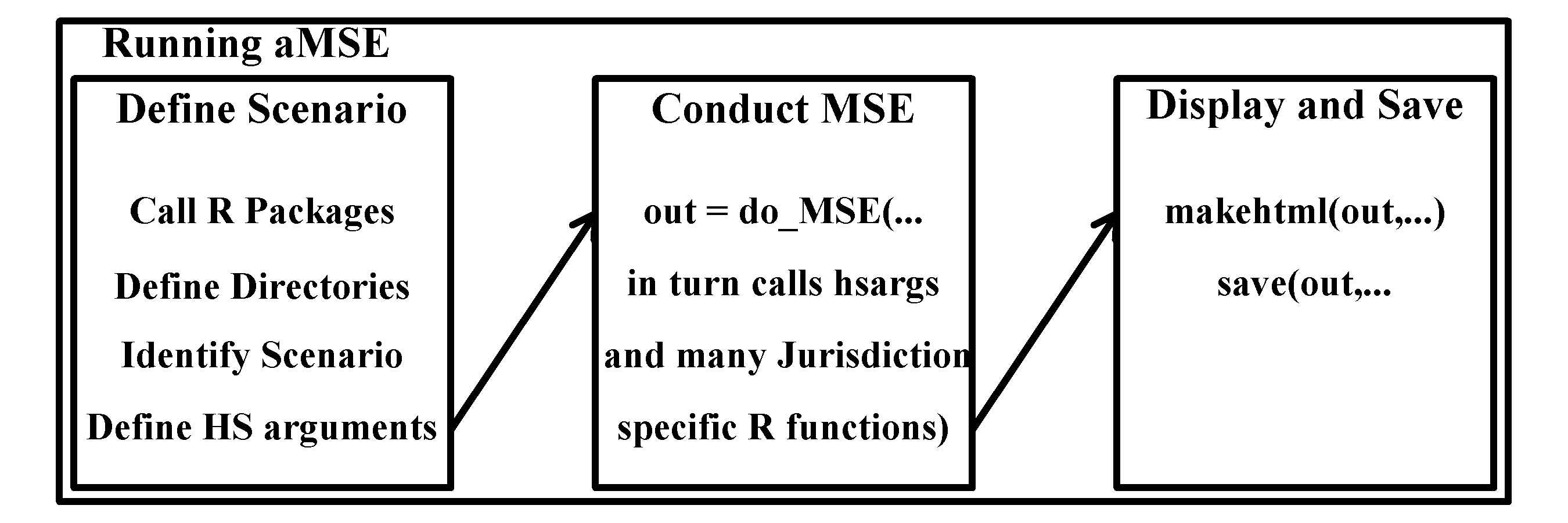
Diagrammatically, the process of running the aMSE software can be summarized as in Figure 3.2, although a verbal description and example R code are also given below.
First one sets up R options (if desired), calls the required libraries, and sets up the directory information:
options("show.signif.stars"=FALSE, # some R options I find helpful
        "stringsAsFactors"=FALSE,  # now a default in R4
        "max.print"=50000,
        "width"=240)
suppressPackageStartupMessages({  # declare libraries -------------
  # this is the minimum, of course others can be added if desired
  library(aMSE)
  library(EGHS)     # obviously only if using the Tasmanian HS
  library(codeutils)
  library(hplot)
  library(makehtml)
  library(knitr)
})
# OBVIOUSLY, modify the rundir definition to suit your own setup!!!
prefixdir <- pathtopath(getDBdir(),"A_codeR/aMSEGuide/runs/")
postfixdir <- "EG"     # a descriptive name for the rundir
rundir <- pathtopath(prefixdir,postfixdir) # define rundir
startime <- Sys.time() # to document the time taken
verbose <- TRUE        # send messages to the console about the run progress
controlfile <- paste0("control",postfixdir,".csv") # match control file name
outdir <- "C:/aMSE_scenarios/EG/"   # storage on a non-cloud hard-drive
confirmdir(rundir,ask=FALSE)   # make rundir if it does not exist
c:/Users/MalcolmHaddon/DropBox/A_codeR/aMSEGuide/runs/EG already exists confirmdir(outdir,ask=FALSE) # to be interactive needs ask = TRUEC:/aMSE_scenarios/EG/ already exists 3.3.2 Making the control and data files
Now we can generate the control and the two data file using aMSE template functions. If these files already exist then, obviously, we do not need to run this code again.
controlfile <- "controlEG.csv" # default example file name, change it as needed
# Now make the controlfile. Read the help file using ?ctrlfiletemplate. This
# explains what the devrec argument is all about.
ctrlfiletemplate(indir=rundir,filename=controlfile,devrec=0)
# Within controlfile, the default data file name is 'saudatapostfixdir.csv'. If
# you want to call it something else (maybe aloysius.csv or machynlleth.csv?)
# then edit the seventh line of the controlfile that holds the definition
# of the name of the SAU data file, and change it in this code.
datafiletemplate(indir=rundir,filename="saudataEG.csv")
# The program also needs some length composition data. For this we are going
# to use one of the inbuilt data-sets called 'lfs' (see its help). The default
# filen is already written into the controlfile. Change that as necessary.
data(lfs)
writecompdata(indir=rundir,lfs,filen="lf_WZ90-20.csv")
# dir(rundir)  # listing the contents of rundir can be a useful check
I recommend that you take a look at the contents of these newly generated files (either in RStudio or Excel, though Excel is best avoided), which will be found in EG, but, for now, do not alter anything, although if you do (perhaps the data file name) be sure to re-save it as a .CSV file and not an .XLSX file. Full details of these files are given in the The Input Files section of the documentation. For now, the user should know that the scenario includes a natural mortality = 0.15, a recruitment steepness = 0.7, and a cpue hyper-stability lambda = 0.75. The latter implies that the dynamics are affected by hyper-stable CPUE rather than the more classical assumption of a linear relationship between CPUE and exploitable biomass (the assumption of linearity may be common and classical, but it is incorrect for abalone and lots of other species).
3.3.3 The HS Package or JurisdictionHS.R File
Here we are using the EGHS R package, and the default hsargs (see code chunk below). If an R package has been developed that implements a harvest strategy for a specific jurisdiction, it will need its own set of hsargs. The functions that are used to define the harvest strategy being tested can be read in via a source R file, or if an R package exists, the relevant library(s) loaded.
# In Tasmania, the HS is included in a package called EGHS, and this
# contains all the required functions.
# Alternatively use source(“pathtoafilecontainingtheHSfunctions.R”)
# But, if the EGHS package is used instead of a source file, we still need
# the global object hsargs, which contains the settings used by the the
# Tasmanian HS. For details of hsargs, see the documentation for ?EGHS or
# for whichever HS you are exploring.

hsargs <- list(mult=0.1, #expansion factor for cpue range when calc the targqnt
               wid = 4, # number of years in the grad4 PM
               targqnt = 0.55, # quantile defining the cpue target
               maxtarg = c(150,150,150,150,150,150,150,150), # max cpue Target
               pmwts = c(0.65,0.25,0.1),  # relative weights of PMs
               hcr = c(0.25,0.75,0.8,0.85,0.9,1,1.05,1.1,1.15,1.2), # hcr mults
               hcrm3 = c(0.25,0.75,0.8,0.85,0.9,1,1.1,1.2,1.25,1.3),# mr 3
               startCE = 2000, # used in constant reference period HS
               endCE = 2019,   # used in constant reference period HS
               metRunder = 0,  # should the metarules be used. 0 = No
               metRover = 0,   # use metarules 0 = No
               decrement=1, # use fishery data up to the end of the time series
               pmwtSwitch = 0, # n years after reaching the targCE to replace
               stablewts = c(0.8, 0.15, 0.05), # pmwts with stablewts mr3
               hcrname="constantrefhcr",     # the name of the HCR used
               printmat=NULL) # something needed for some HS, not TAS
If using a jurisdictionHS.R source file, then it needs to contain a number of specific functions and constants, even where some may, in fact, do nothing:
tasFIS <- function(x) { # currently no FIS data is used in TAS
  return(NULL)          # though this may change
}
For full details see the JurisdictionHS_Requirements section.
3.4 Running do_Conditioning
Once setup with all the required files and packages, one would normally attempt to condition the model by changing input parameters so that it generates simulated dynamics that more closely follow those observed in the real fishery. For example, it is possible to modify recruitment deviates in particular years, which would modify the available exploitable biomass in later years, which, in turn, will change the predicted CPUE and associated size-composition of catches, with the intention of improving the match between the observed and that predicted by the operating model. However, if, when running the ctrlfiletemplate function, you used the devrec=0 argument (as we did), then the recruitment deviates for the western zone, under a scenario of natural mortality M = 0.15, recruitment steepness = 0.75, and a hyperstability parameter lambda = 0.75, have already been optimized using the sizemod size-based modelling package to provide the best statistical fit between the observed and predicted CPUE and the observed size-composition of the catch and that predicted by the model (see Using_sizemod_to_condition_the_SAU).
Despite having the operating model already conditioned, here we will run the code needed to condition the model on the historical data to illustrate what the outputs will look like. The code in the next block automatically generates a set of web-pages using HTML and CSS to layout and display the results. If you run this code while having Windows Explorer (or whatever equivalent you are using on your machine) open on your rundir you should see the generation of an array of files prior to the web-pages being opened automatically in a browser. If you were to set the argument openfile = FALSE then the browser would not be activated, but you could open it all by double clicking on the EG.html file within the EG directory. Alternatively, one can enter, into the RStudio console, browseURL(pathtopath(rundir,“EG.html”)).
prodout <- FALSE  # no estimation of production properties saves time but
# this runs the MSE on a control rule that uses no meta-rules. It will be
# compared with scenarios that include meta-rules in a later example.
out <- do_condition(rundir,controlfile,  # controlfile defined above
                    calcpopC=calcexpectpopC,  # from EGHS
                    verbose = TRUE,
                    doproduct = prodout, # prodout=FALSE, no details re MSY
                    dohistoric=TRUE,
                    matureL = c(70, 200), # length range for maturity plots
                    wtatL = c(80, 200), # lengths for weight-at-length plots
                    mincount=120,  # minimum obs for including length comps
                    uplimH=0.35,   # not used because doproduct=FALSE
                    incH=0.005,
                    deleteyrs=0,  # all length comp years used
                    prodpops=NULL) # no individual pop producivity plotted
All required files appear to be present
Files read, now making zone
Time difference of 0.7475371 secsConditioning on the Fishery data makeoutput(out,rundir,postfixdir,controlfile,hsfile="EGHS Package",
doproject=prodout,openfile=TRUE,verbose=FALSE)The local web page displaying the output has a number of tabs. The condition tab illustrates the match between the observed cpue and that predicted by the operating model, while the predictedcatchN tab illustrates the match between the observed size-composition of the catches and the predicted values. It is clear that those sau with small sample sizes of size-composition data only have a relatively poor model fits in some years.
Each of these tabs are repeated when running the do_MSE() function so more detailed descriptions of each tab will be given in the next section where the MSE will be run using the default Tasmanian harvest strategy. Note that the main page is named ‘EG’, which reflects the fact that the scenario webpage top-lvel tab is named after the postfixdir.
3.5 Running do_MSE
Once conditioning the model has been completed to the degree desired, one can run projections for a specific management scenario with the simulated abalone zone’s management being determined by the harvest strategy as implemented in EGHS (see the discussion concerning the spectrum of options relating to conditioning operating models and how that related to the specific objectives of the simulation testing being undertaken).
If one keeps an Explorer window open looking at rundir, the addition of different files can be watched in real time. The MSE can be run using the following code (I suggest you examine the help files for any functions new to you). do_MSE() provides notifications to the console about the progress of calculations if ‘verbose=TRUE’ is set. The checkhsargs() function is defined to examine hsargs but is only valid for the TAS EHS. Any other jurisdiction would need to write an equivalent function to interact with their own HS and hsargs requirements.
checkhsargs(hsargs) # lists chosen options before run, only for TASThe hcr being used is: constantrefhcr
hsargs$startCE and hsargs$endCE are used to define the reference periods for each sau
# ?do_MSE provides more detailed descriptions of each function argument
# see EGHS package for help with the HS functions
# do_MSE function can take a few minutes to run so be patient
out <- do_MSE(rundir,controlfile, # already known
              hsargs=hsargs,    # defined as global object
              hcrfun=constantrefhcr,   # the main HS function
              sampleCE=tasCPUE, # processes cpue data
              sampleFIS=tasFIS, # processes FIS data (if any)
              sampleNaS=tasNaS, # processes Numbers-at-Size data
              getdata=tasdata,  # extracts the data from the zoneDP object
              calcpopC=calcexpectpopC, #distributes catches to populations
              makeouthcr=makeouthcr, # generates updateable HS output object
              fleetdyn=NULL,   # only used in SA and VIC so far
              scoreplot=plotfinalscores, # a function to plot HS scores
              plotmultflags=plotmultandflags, # function to plot multipliers
              interimout="", # save the results after projecting,
              varyrs=7, # years prior to projections for random recdevs
              startyr=48, # in plots of projections what year to start
              verbose=TRUE, # send progress reports to the console
              ndiagprojs=4, # individual trajectories in DiagProj plots
              cutcatchN = 56,  # cut size-at-catch array < class = 112mm
              matureL = c(70, 200), # length range for maturity plots
              wtatL = c(50, 200),   # length range for weight-at-length plots
              mincount = 120,   # minimum sample size in size-composition data
              includeNAS = FALSE, #include the numbers-at-size in saved output?
              depensate=0, #will depensation occur? see do_MSE help for details
              kobeRP=c(0.4,0.2,0.15), # ref points for a kobe-like phase plot
              nasInterval=5,  # year interval to use when plotting pred NaS
              minsizecomp=c(100,135), #min size for pred sizes, min for catches
              uplimH=0.35,incH=0.005, #H range when estimating productivity
              deleteyrs=0)    # all length comp years used
All required files appear to be present
Files read, now making zone
Now estimating population productivity between H 0.005 and 0.35
makeequilzone 27.23758 secs Conditioning on the Fishery data
dohistoricC 1.202465 secs Conditioning plots completed 1.615715 secs Preparing for the projections
Projection preparation completed 10.51057 secs
Doing projections
2021 2022 2023 2024 2025 2026 2027 2028 2029 2030 2031 2032 2033 2034 2035 2036 2037 2038 2039 2040 2041 2042 2043 2044 2045 2046 2047 2048 2049 2050
All projections finished 1.670104 mins
Now generating final plots and tables
Starting the sau related plots Finished all sau plots 15.0005 secs
Starting size-composition plots Finished size-composition plots 8.004758 secs Plotting fishery information hsargs.txt saved to rundir
plotting HS performance statistics plotting Population level dynamics All plots and tables completed 16.11022 secs You could check out the list of files in rundir using dir(rundir). If the numbers-at-size are saved (includeNAS=TRUE) the out object can be gigabytes rather than megabytes. Best to only use this option when making a final scenario run.
The do_MSE() function currently requires 29 input parmeters.The rundir and controlfile were defined earlier, the remaining 27 arguments are new and are described in the help page for do_MSE() (?do_MSE).
A flag can be set (verbose) to determine whether to have updates on progress sent to the console as they were above. This can be helpful, especially during development. While you should examine the help for do_MSE() some of the more important arguments will be considered here. The function makes great use of R’s ability to use function names as arguments to other functions. In that way, while we have standard names for functions within do_MSE() one can point each of those to custom functions devised for each jurisdiction’s approach to managing its abalone stocks. Just as each jurisdiction will require hsargs to have a different set of components, the arguments listed here all require functions to be written for each jurisdiction to match the requirements of each HS.
• hcrfun=constantrefhcr, is the main function driving the HS. It gathers all the inputs and is expected to output everything wanted from the HS. In the case of Tasmania, the minimum would be the acatch for each SAU. In fact, many more outputs are output and stored (in outhcr) so that the HS performance can be plotted and monitored.
• sampleCE=tasCPUE, controls how the CPUE data from the simulations are smapled and processed prior to use within the HS (see the R code by typing tasCPUE into the console with no following brackets).
• sampleFIS=tasFIS, similarly this function would process any FIS data is any were available.
• sampleNaS=tasNaS, processes the Numbers-at-Size data from the populations to generate the predicted number-at-size in the catch.
• getdata=tasdata, extracts the data from the zoneDP object, which is used to hold the dynamics of the dynamic zone during projections.
• calcpopC=calcexpectpopC, once the acatch (or TACC) is known then this function is used to distribute that catch across the populations within each SAU (needed even where management does not use SAU scale catch allocation.
• makeouthcr=makeouthcr, this is used in the function doprojections where it is input into hcrfun (here that is constantrefhcr), which outputs an updated version. A the end of the projections it will therefore contain all the outputs from hcrfun ready for characterization.
• fleetdyn=NULL, where the default fleet dynamics is not used (which predicts the catch from each SAU based on available exploitable biomass plus noise) this is where a custom function can be input (this is needed in South Australia)
• scoreplot=plotfinalscores, a jurisdiction specific function to plot HS scores
• plotmultflags=plotmultandflags, a function to plot eh catch multipliers as implemented in each jurisdiction.
When you run this do_MSE() code, in fact it will be doing rather a lot of work, even though in this instance it is only running 100 replicates (more normally do 250 or 500). Apart from the results contained in the multiple .png files (plots), .csv files (tables), and some other .csv files, all the results can be found in the out object associated with the do_MSE() statement.
str1(out) # function from codeutils = str(out,max.levels=1)List of 30
$ tottime : 'difftime' num 2.787
$ runtime : POSIXct[1:1], format: "2025-09-12 10:37:46"
$ starttime : POSIXct[1:1], format: "2025-09-12 10:34:59"
$ glb :List of 22
$ ctrl :List of 13
$ zoneCP :List of 56
$ zoneD :List of 14
$ zoneDD :List of 14
$ zoneDP :List of 14
$ NAS : NULL
$ projC :List of 6
$ condC :List of 15
$ sauout :List of 10
$ outzone :List of 13
$ production : num [1:71, 1:6, 1:56] 256 245 235 225 216 ...
$ condout :List of 2
$ saucomp : num [1:105, 1:30, 1:8] 6.92e-54 9.66e-52 1.00e-49 7.49e-48 4.05e-46 ...
$ HSstats :List of 2
$ saudat : num [1:33, 1:8] 21.5 0.3 130 1 54.3 ...
$ constants : num [1:34, 1:56] 6 21.5 0.3 130 1 ...
$ hsargs :List of 16
$ sauprod :List of 3
$ zonesummary :List of 2
$ kobedata : num [1:8, 1:4] 0.33 0.449 0.259 0.242 0.313 ...
$ outhcr :List of 8
$ scoremed : num [1:30, 1:7] 42.8 35.4 31.5 31.3 33.4 ...
$ popmedcatch :List of 8
$ popmedcpue :List of 8
$ popmeddepleB:List of 8
$ pops : num [1:56, 1:26] 1 2 3 4 5 6 7 8 9 10 ...Many of these objects are lists and so one might use str() or str2() to examine their structure and contents, but this has been done for you in the R_Object_Structure_of_Output section of the documentation (though you could/should still try it yourself). The many plots and tables produced remain only a start. Any number of further plots and tables can be produced from what is already there but especially when alternative scenarios are compared. So, knowing the object structure of what comes out is extremely helpful.
Most of the analyses we can see are conducted at the primary grouping level (i.e. the sau level for EGHS). Thus, the main objects for initial study would be the sauout, NAS, outzone, and even the zoneDP objects (population level dynamics). See the R_Object_Structure_of_Output section for more details.
You should run the dir(rundir) to see how many files have been created by the MSE ready for use.
We can now construct the internal web-page to display results. If you set the argument ‘openfile=TRUE’ then the internal website will open automatically. If set to FALSE then you would need to open the rundir and double-click the scenario html file. For example, if your scenario is called EG then you would click on EG.html, alternatively, one can enter, into the RStudio console, browseURL(paste0(rundir,“.html”)), which will automatically use the latest analysis conducted into rundir.
makeoutput(out,rundir,postfixdir,controlfile,
           hsfile="EGHS Package",openfile=TRUE,verbose=FALSE)
Obviously, this is a multi-faceted summary of what has been done. It includes the pages from do_condition plus many more.
3.5.1 Save Outputs for later Comparison
The primary intent of the aMSE software is to make comparisons between alternative harvest strategy scenarios. For this it is necessary to save the out objects (which, without the NAS object are hundreds of mega-bytes and with the NAS object can be giga-bytes). Because of their size it is best to store these on a local and fast hard drive so that when making comparisons the separate out object for each scenario can be examined and the outcomes compared. Here we illustrate the required R code and we will use the results later in the documentation when comparing the basecase with alternatives.
save(out,file=pathtopath(outdir,paste0(postfixdir,".RData")))3.5.2 Home Page
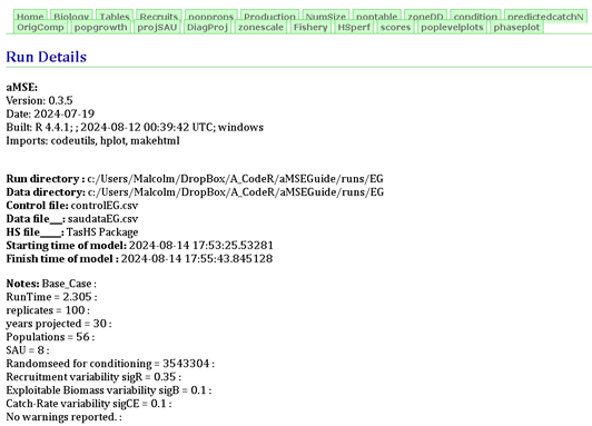
The Home tab contains lines of information concerning the particular scenario run of the MSE. This information includes the directories used, the files used, some details of the run (number of replicates, years projected, number of populations and sau) but especially the randomseed used when generating the different populations within the sau. If that randomseed, which is set in the controlfile, is altered one would expect the complete conditioning to be different as many of the properties of each population would change slightly. What this number does is ensure that the same simulated zone is generated each time a scenario is run.
In the following pages are a wide variety of results and outputs but, of course, any number of extra, additional, or alternative plots and tables could be included on each page (although that would entail updating the do_MSE() function, or functions it refers to). Each figure and table caption contains the name of the .png or csv file from which it is produced should the figure or table be needed for any other purpose. Clicking on any figure will enlarge it for ease of examination (use the return arrow at top left in the browser to return to the original page). In the sections below describing each tab a figure is given illustrating at least one plot from each tab. See the respective tab for the related caption.
3.5.3 Biology Page
This contains plots of the maturity-at-length curves, weight-at-size curves, and emergence-at-size curves for each population in each SAU. For each metric, there is a pane of plots for each SAU, each of which contains indicators for every population in that SAU
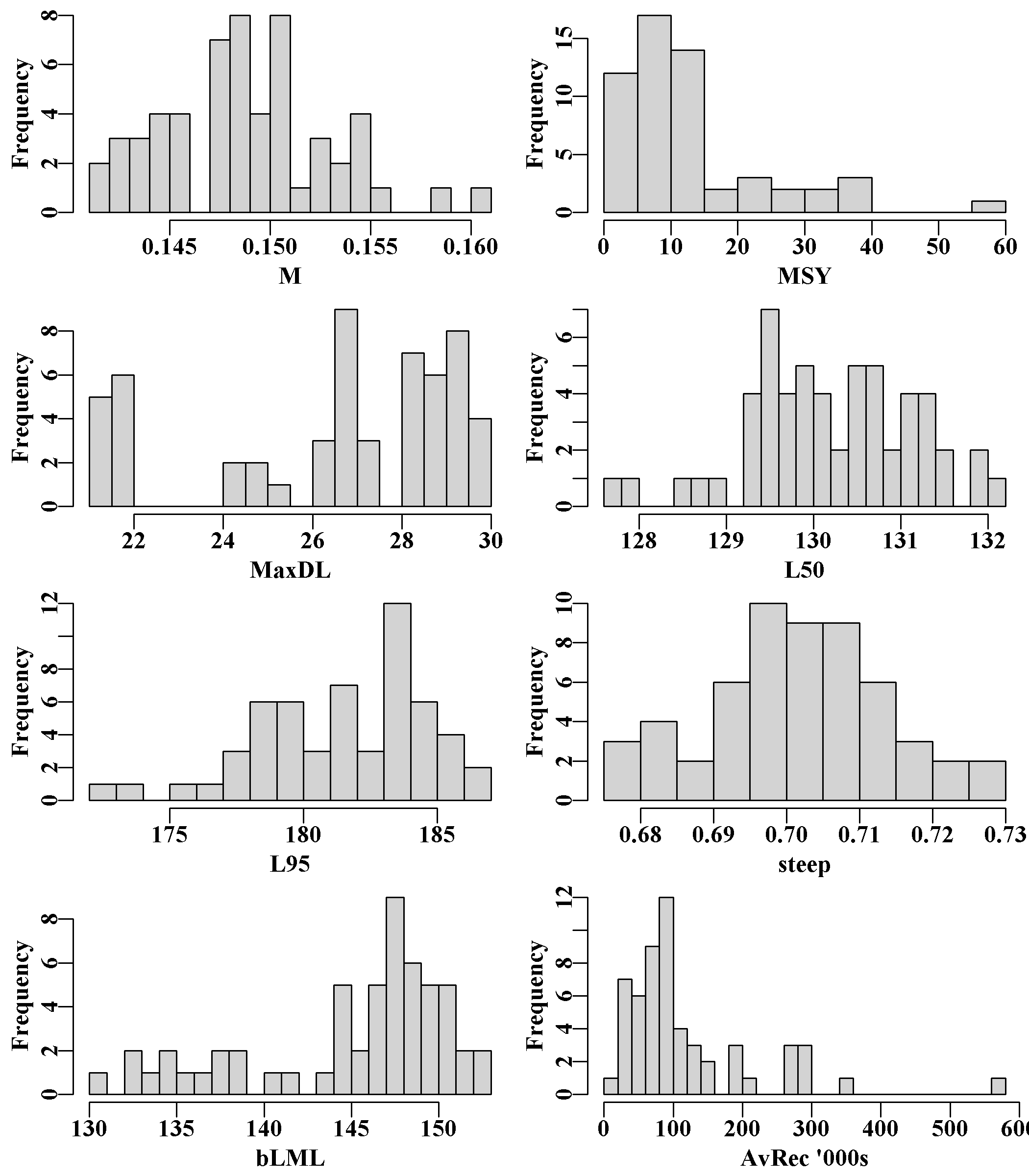
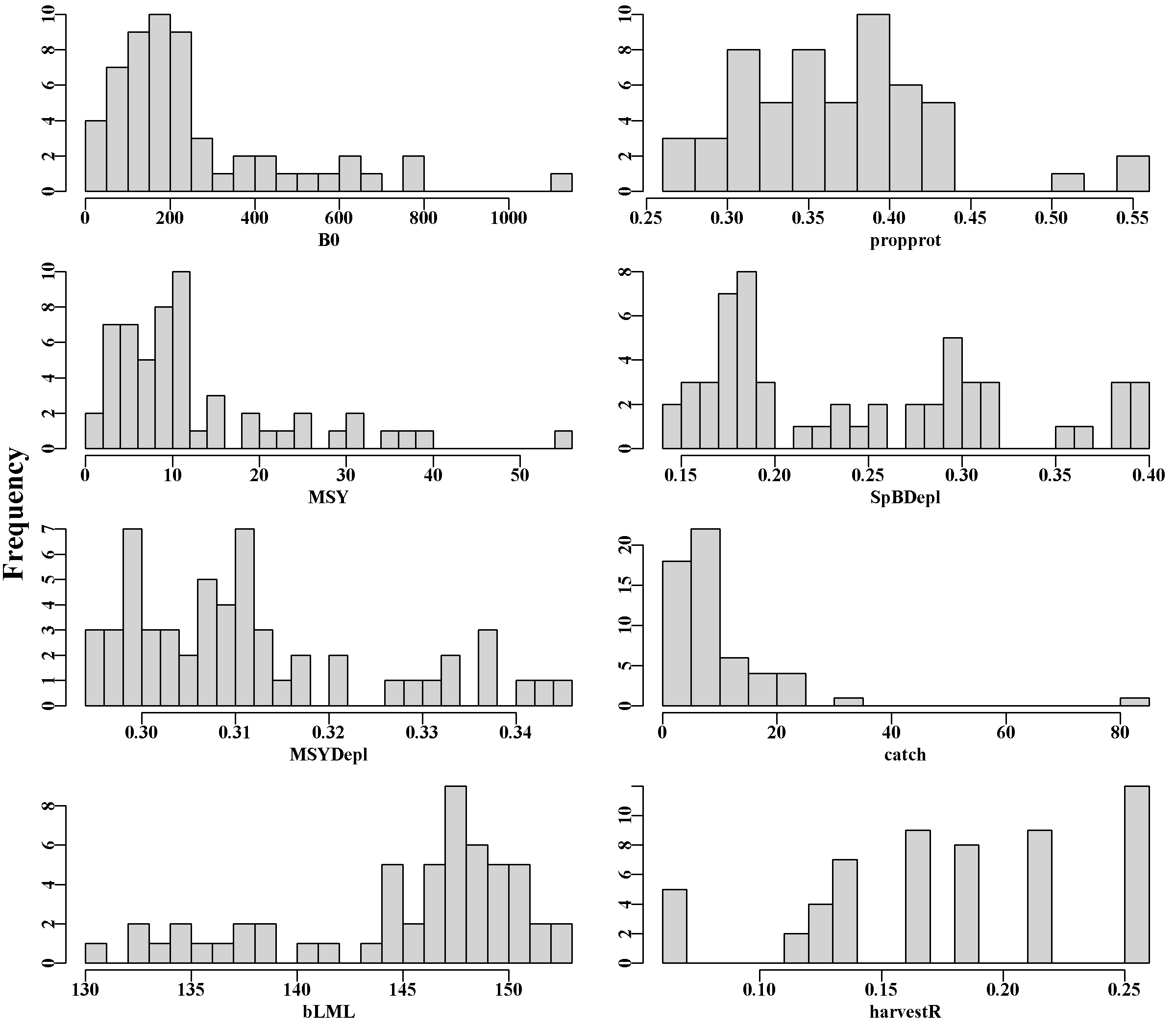
The final eight histograms of biological properties illustrate the variation among population’s for their values of natural mortality, M, the MaxDL, L95 and L50 growth parameters across all SAU and populations. There are also histograms of each population’s MSY, steepness, and the biological LML (size-at-maturity plus two years’ growth. Finally, AvRec, the unfished recruitment, are also variable, but this reflects the fact that in each sau only a proportion of the total sau AvRec is allocated to each population. There is almost no random variation in the AvRec values between R runs as the standard deviation is set to 1e-05 in each case (because the AvRec value is fitted within sizemod.
3.5.4 Tables Page
Currently, this holds only two tables, the first being the productivity properties of each sau (B0, MSY, etc), and the second being the tabulated contents of zonebiology.csv. This represents the various actual values for an array of biologically important variables (including those plotted as histograms on the Biology page), all by population. The input constants for population biological properties are derived from adding random variation to the SAU scale property values.
| sau6 | sau7 | sau8 | sau9 | sau10 | sau11 | sau12 | sau13 | |
|---|---|---|---|---|---|---|---|---|
| R0 | 258881 | 461928 | 239640 | 1058383 | 836448 | 1720648 | 1546067 | 583240 |
| B0 | 438.882 | 872.171 | 524.479 | 2438.878 | 2071.964 | 4152.789 | 3126.261 | 915.911 |
| ExB0 | 414.822 | 845.227 | 522.023 | 2450.284 | 2117.053 | 4164.472 | 3203.565 | 869.511 |
| MSY | 20.283 | 43.738 | 24.955 | 122.512 | 102.811 | 207.707 | 156.662 | 41.758 |
| steep | 0.691 | 0.705 | 0.7 | 0.698 | 0.707 | 0.702 | 0.705 | 0.695 |
3.5.5 Recruits Page
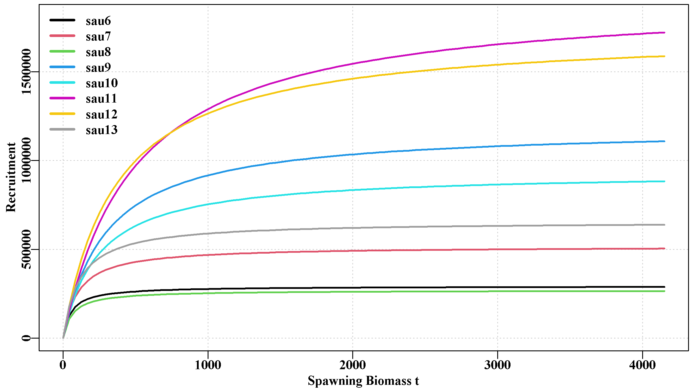
This holds two plots. The first is a representation of the stock recruitment relationship for each sau, all on one plot. This illustrates how different each sau is in terms of productivity. The second plot includes a plot of the stock-recruitment relationships of each population within each sau, which illustrates the variation apparent in the defined populations. Each plot has its own y-axis scale, so care is needed with interpretation.
3.5.6 popprops Page
Tabulates some of the properties of the individual populations within each sau. Currently this reflects only the proportion of the average recruitment by sau allocated to each population, which repeats what is found in the saudataEG.csv file.
3.5.7 Production Page
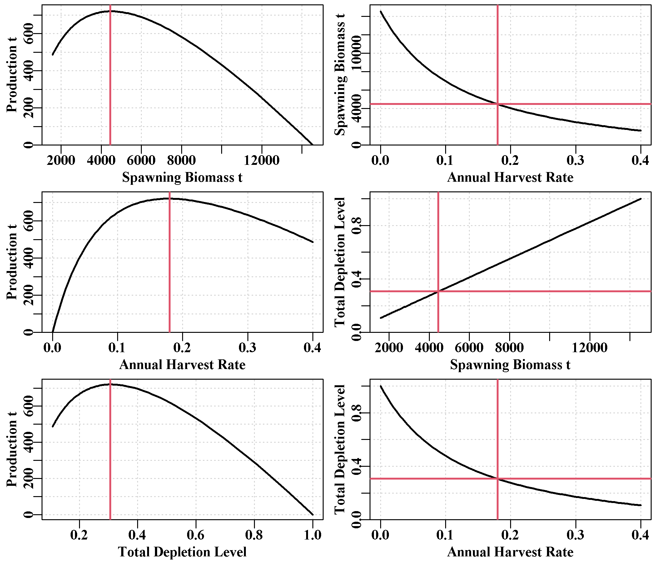
As the name suggests, this tab provides figures and tables realting to productivity. It has a plot of the production curve relative to expected CPUE for each sau, including estimates of the MSY and the predicted CPUE at MSY. The second plot is of the productivity curves for the whole zone. This more complex plot could be generated for each sau as desired using the production array (try str1(out$production)).
Finally, there is a small 5 x number-of-sau matrix of \(B0\), \(B_{MSY}\), \(MSY\), \(D_{MSY}\) (depletion at MSY), and \(CE_{MSY}\) (predicted cpue at \(B_{MSY}\)) for each sau. This has extra information to the first table in the Tables page.
3.5.8 NumSize Page
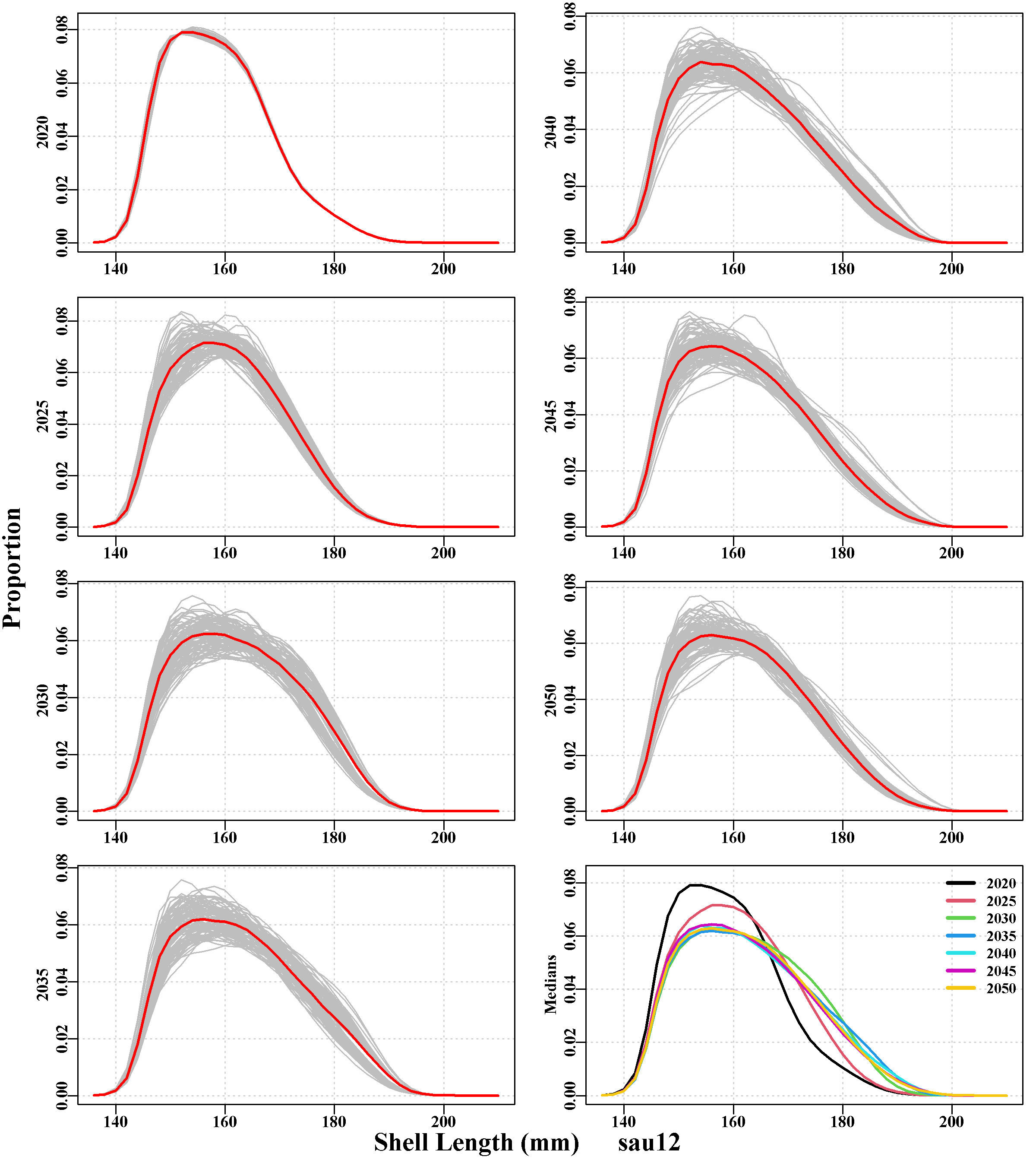
This remains in need of further development. It includes a single plot containing the expected equilibrium, unfished numbers-at-size for the whole zone, and a second plot illustrating the numbers-at-size for each population With 56 populations individual population details cannot be discerned, but it still illustrates the variation in growth, modal progression and productivity among populations). Following the messy all population plot is a separate plot for each SAU, with snapshots of the size distribution of the stock in 5-year steps across the projection period. Following these is a similar set of 5-year snapshots of the size-distribution of each replicate’s catch for each SAU.
3.5.9 poptable Page
This contains the basic biological properties for each of the 56 populations in the example. This is obviously a large table, which is also saved as popprops.csv inside the out object. These values are based on the values provided as input in saudata.csv, with added variation within the range specified.
3.5.10 zoneDD Page
As with any web page on Windows, pressing ‘ctrl +’ increases the size of the contents and ‘ctrl -’ decreases the size. With the figures, each can clicked and they enlarge automatically, at top left is the back arrow that will return one to the broader view (Figure 3.4). Selecting the zoneDD tab leads to a page with a figure made up of histograms of some of the major derived properties of the 56 populations (as in the Biology tab) and then four large tables.
The top table on this tab shows the contents of the propertyDD.csv file now found in rundir, some of which is plotted in Figure 3.9. These are the conditioned emergent properties of each population in the zone. The second is a table of the last ten years of harvest rates during the conditioning for each population from the final_harvestR.csv file. Very high values in any SAU or population indicate a potentially poor fit. In this case there are some values in the first three populations (sau6) above 0.4 in years V2, V4 and V5, but sau6 to sau8 are difficult sau to fit a model to. The third is the table of saudat.csv, which contains the data read in from the saudataEG.csv file for reference. Finally, the fourth table, popdefs.csv, contains the specific parameter values produced for various properties of each population.
3.5.11 condition Page
With the 8 SAU in the Tasmanian conditioning, this tab contains 12 plots and two tables. The first plot compares the observed CPUE for each SAU, from the historical time series input in the control file, with those predicted by the operating model after biological conditioning and fitting the data using the R package sizemod. If you click on the plot in the web-page with your mouse, it will expand to become easier to read the details. Return to the main page using the left arrow (back) at the top of your browser (Figure 3.4). The match between the observed and predicted values, (Figure 3.10) appear very good, although sau8 is clearly a complex situation for any model to fit as since about 2012 the dynamics have been influenced by other factors not in the model.
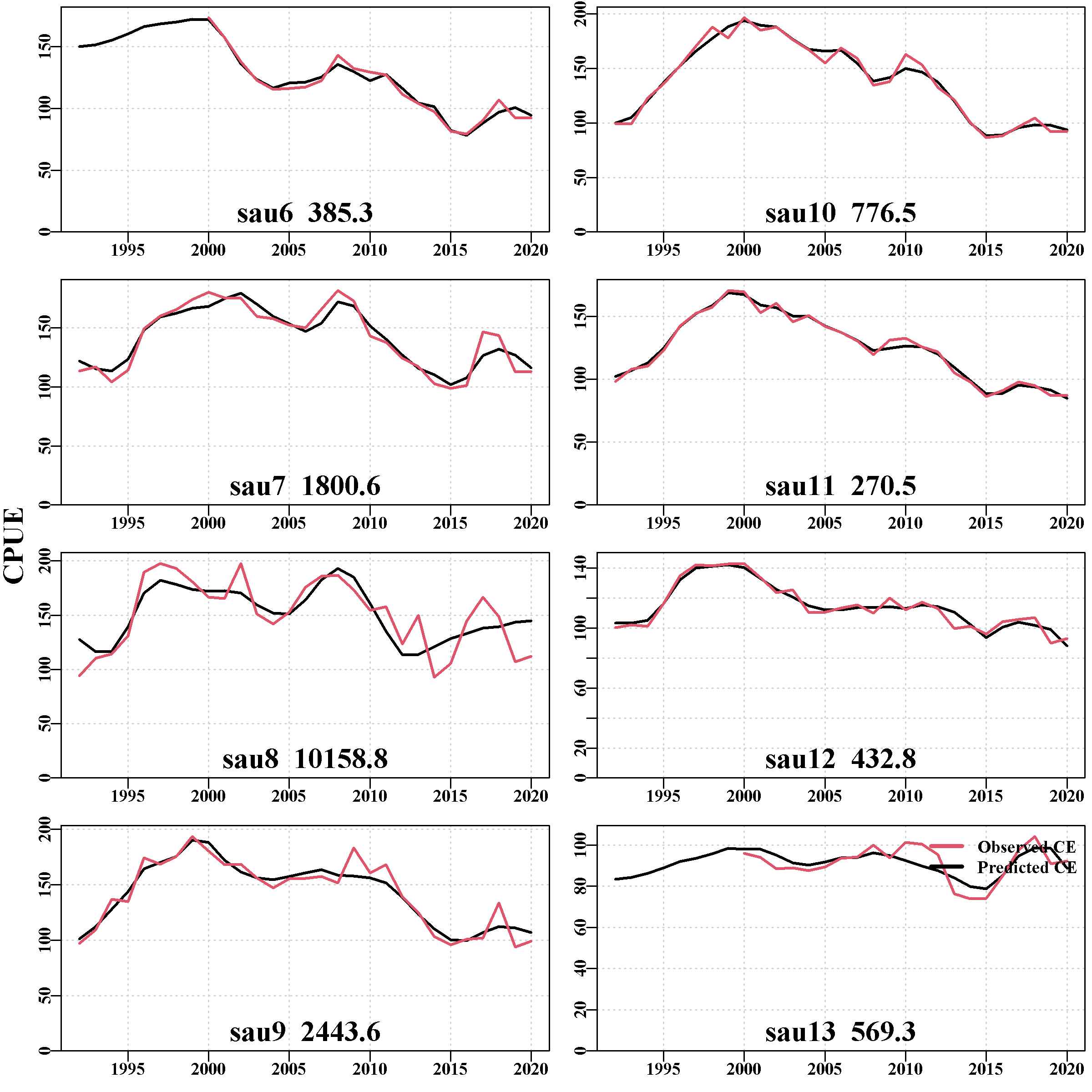
An example of the individual SAU plots is given for SAU 10. Below the comparison of CPUE plot there are 8 plots, one for each sau, illustrating the trajectory of the mature biomass depletion level, the catch through time, the cpue (with the observed values in green), the implied annual harvest rate, the mature biomass (in tonnes), and the implied recruitment level (prior to 1982 and post 2014 are deterministically taken from the stock recruitment curve).
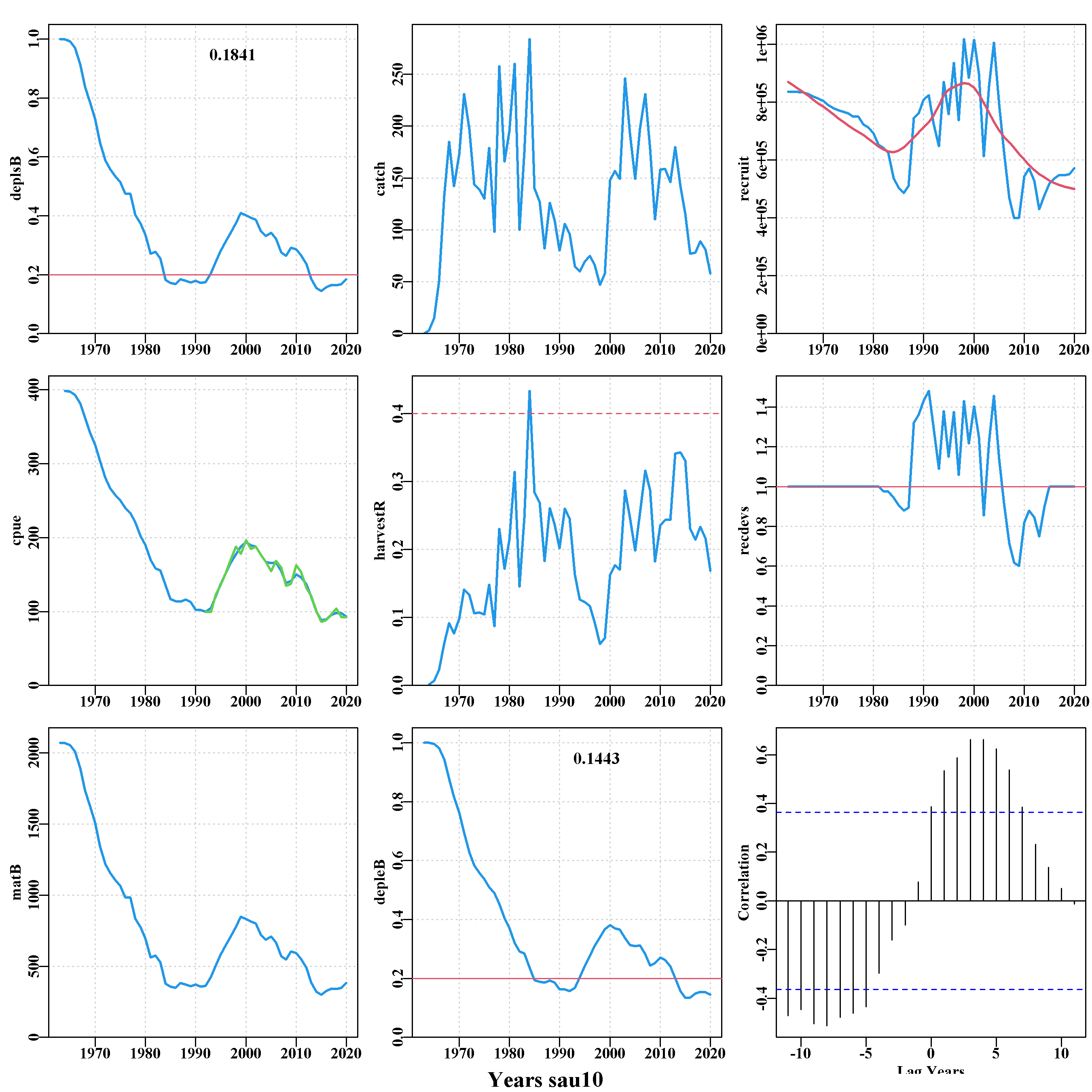
Below the plots for each sau is a summary plot of each recruitment trace used to simplify looking for correlated recruitment events predicted by the model. It is important to remember that the recruitment deviates produced by sizemod and reproduced in aMSE are estimates and not observed data. Nevertheless, it is possible to see repeating patterns of positive and negative recruitment levels between sau. For example, sau10 to sau13 all show a decline prior to 2010 followed by a rise, although the exact timing appears to differ by a year or so between some sau. sau6 and sau13 only have recruitment deviates from 1990 to 2014 because they were only formed in 2000 when zonation was introduced, which limits the data available for conditioning.
The final plot is a histogram of the depletion in the final year of conditioning. This illustrates the effectiveness of including recruitment variation when preparing for the projections (which was set in do_MSE() using the varyrs=7 argument). This figure is then complemented by a table of the quantiles of that final year’s depletion level.
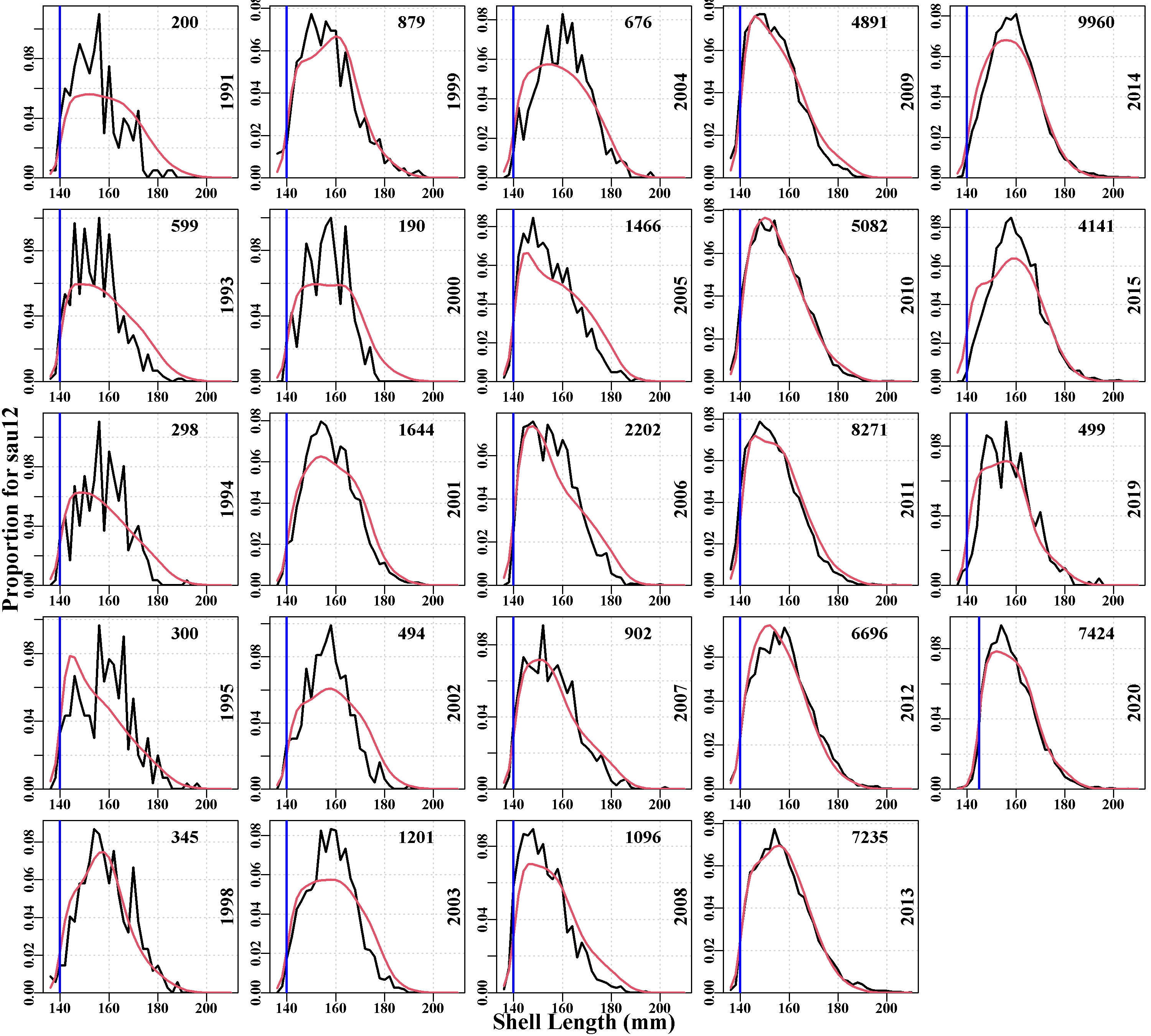
3.5.12 predictedcatchN
Illustrates the fit to the observed numbers-at-size in the catch obtained during the conditioning. The quality of fit is very much affected by the number of observations involved. These plots are for data at the sau scale, so they integrate across however many populations are deemed to make up the sau’s dynamics. Given this is the case, the fit in some cases is remarkably good, for example, in sau11 to sau13, the last plots on the page, the fits to the later samples where sample sizes are large are excellent. sau6 has the least data and generates the worst fit to size-composition data.
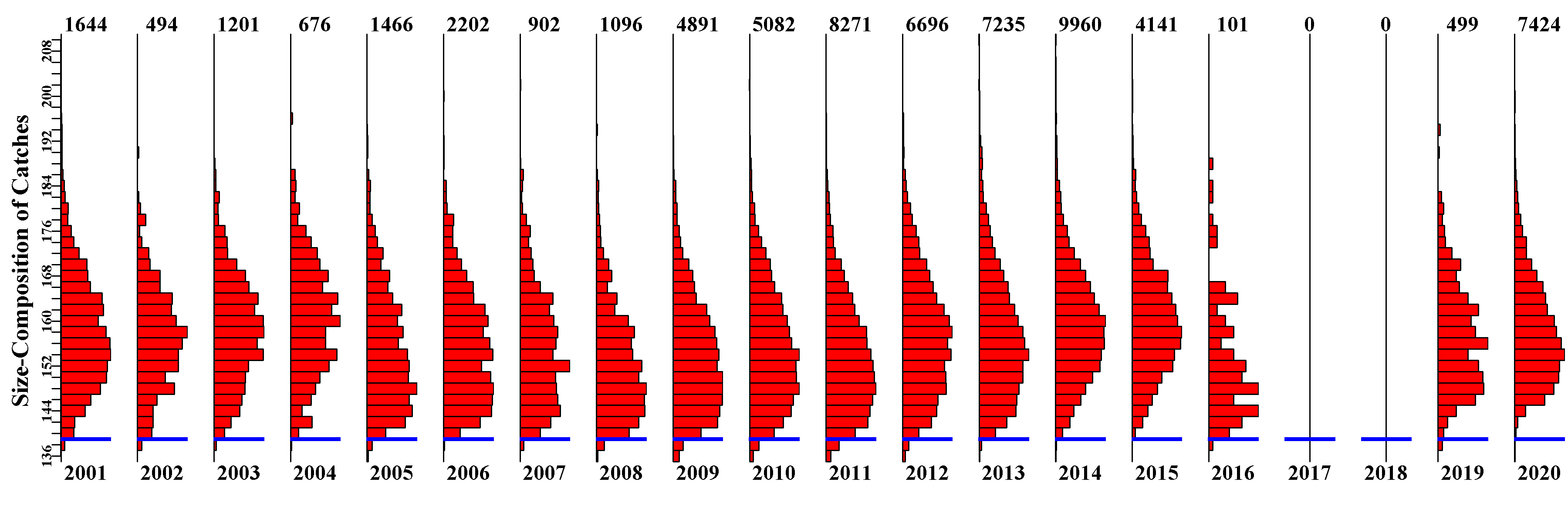
3.5.13 OrigComp Page
Contains plots of the original size-composition of catch data. This is primarily for reference but also provides an image that allows for an appreciation of changes through time and of any gaps in the time-series. Understanding one’s data is vital when attempting to understand how the dynamics in a stock may be changing.
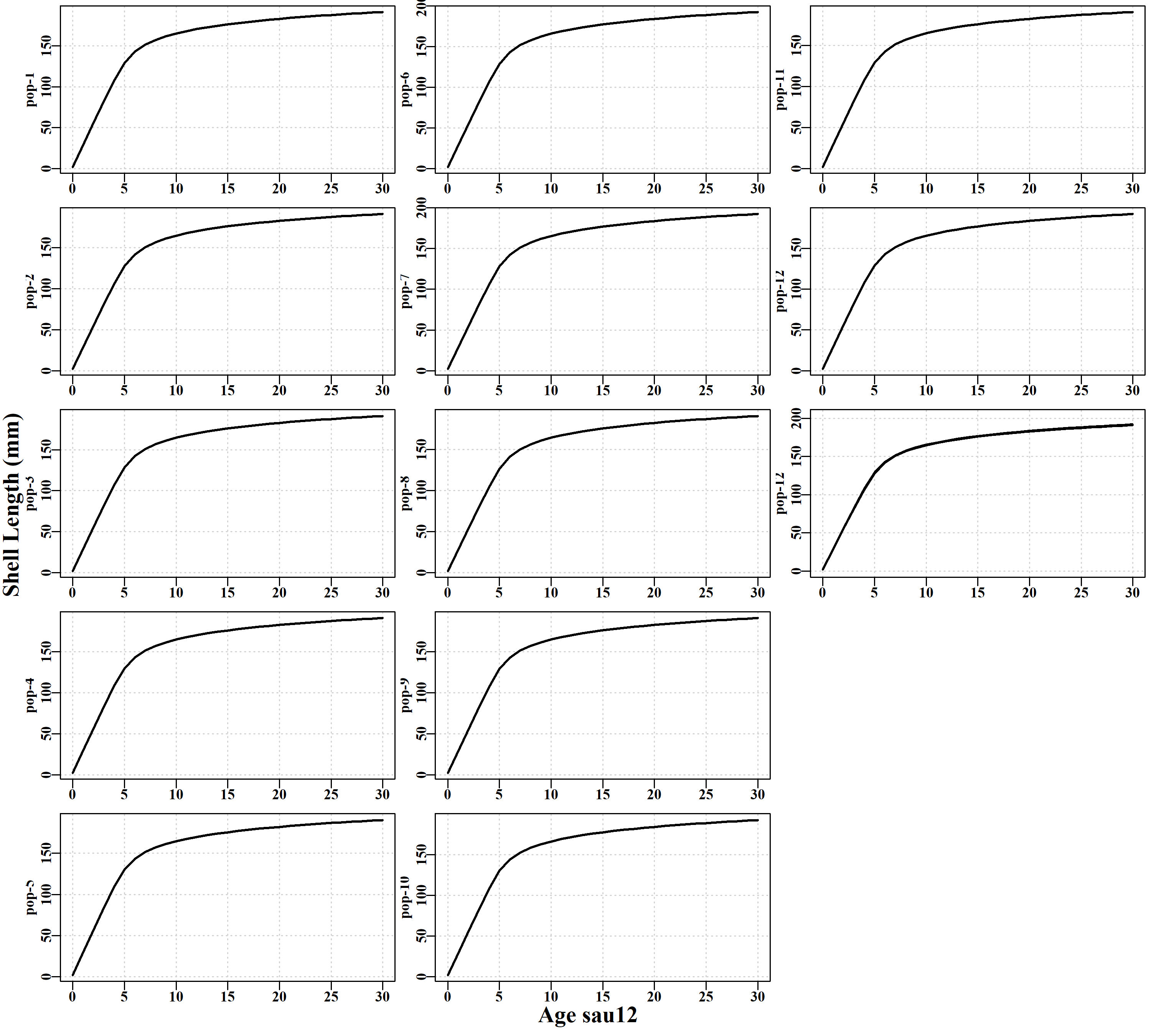
3.5.14 popgrowth Page
Has plots of the individual growth curves expressed in each population within each sau. This enables a better appreciation of the variation in growth included within and between sau.
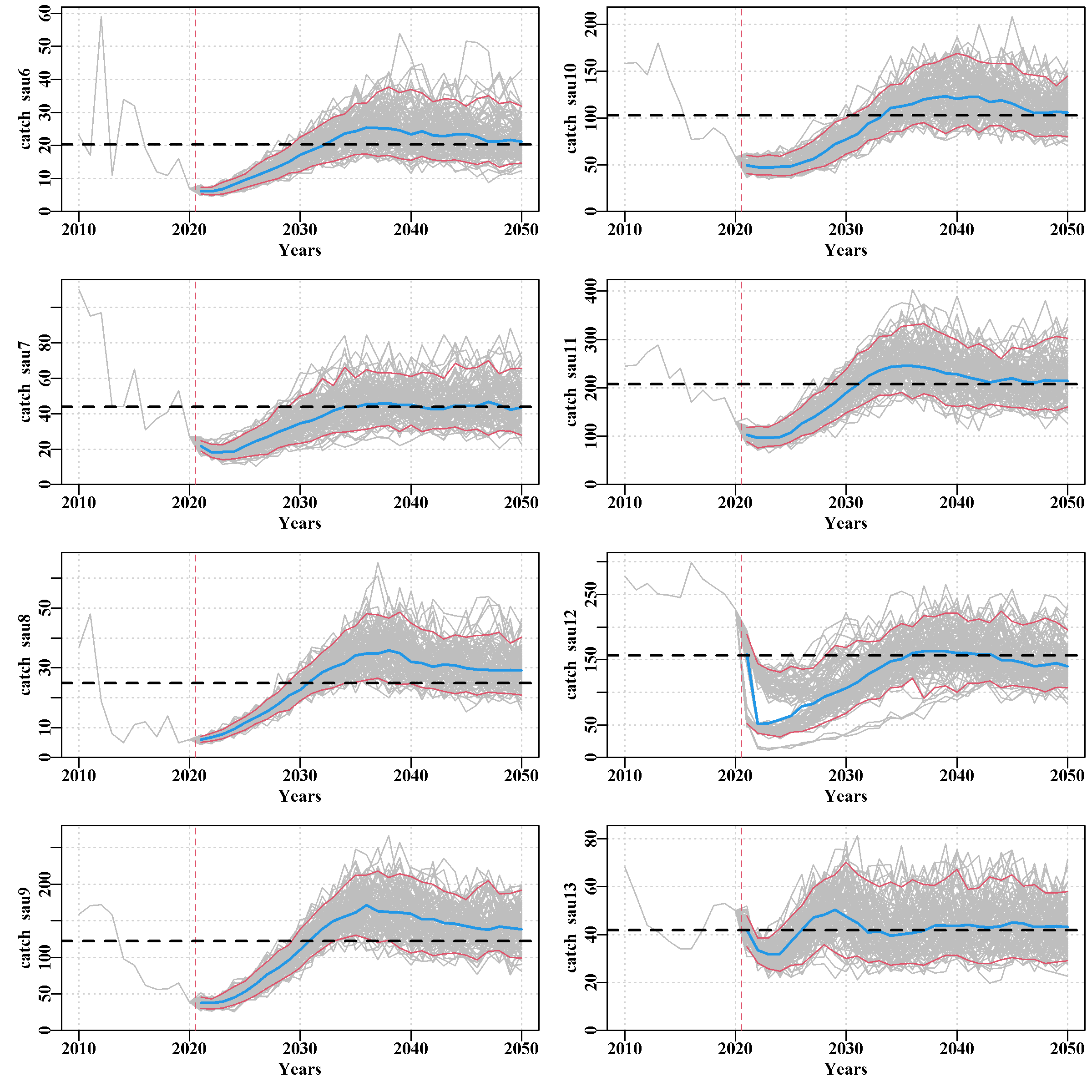
3.5.15 projSAU Page
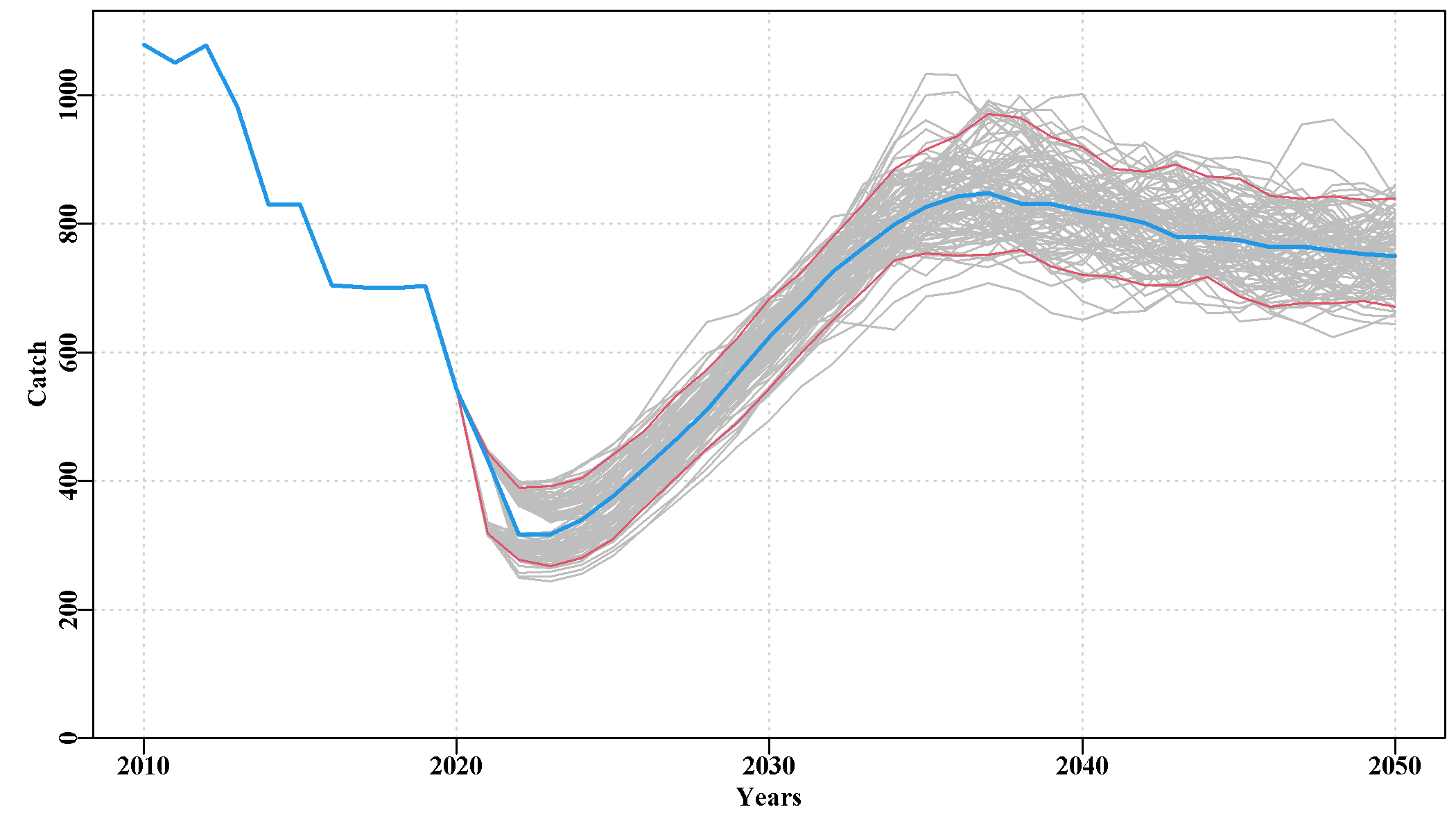
This page illustrates the effect of the harvest strategy on the dynamics of each sau. There are seven plots, the first being for the predicted CPUE by sau, then the predicted actual catch and aspirational catch (the first, not surprisingly, being more variable than the second because that is one source of variation added in the MSE), then comes the mature biomass followed by the exploitable biomass (very similar and currently reflective of the CPUE trends). Finally, comes the predicted recruitment trend and the last plot is of the predicted annual harvest rate.
The grey lines represent the trajectory of individual runs, and illustrate the variation among replicates within each SAU. The each plot also has the median value of replicates (blue line) and the 90th quantile bounds (fine red lines). It is important to appreciate that these are derived values across all replicates, and do not represent an individual run.
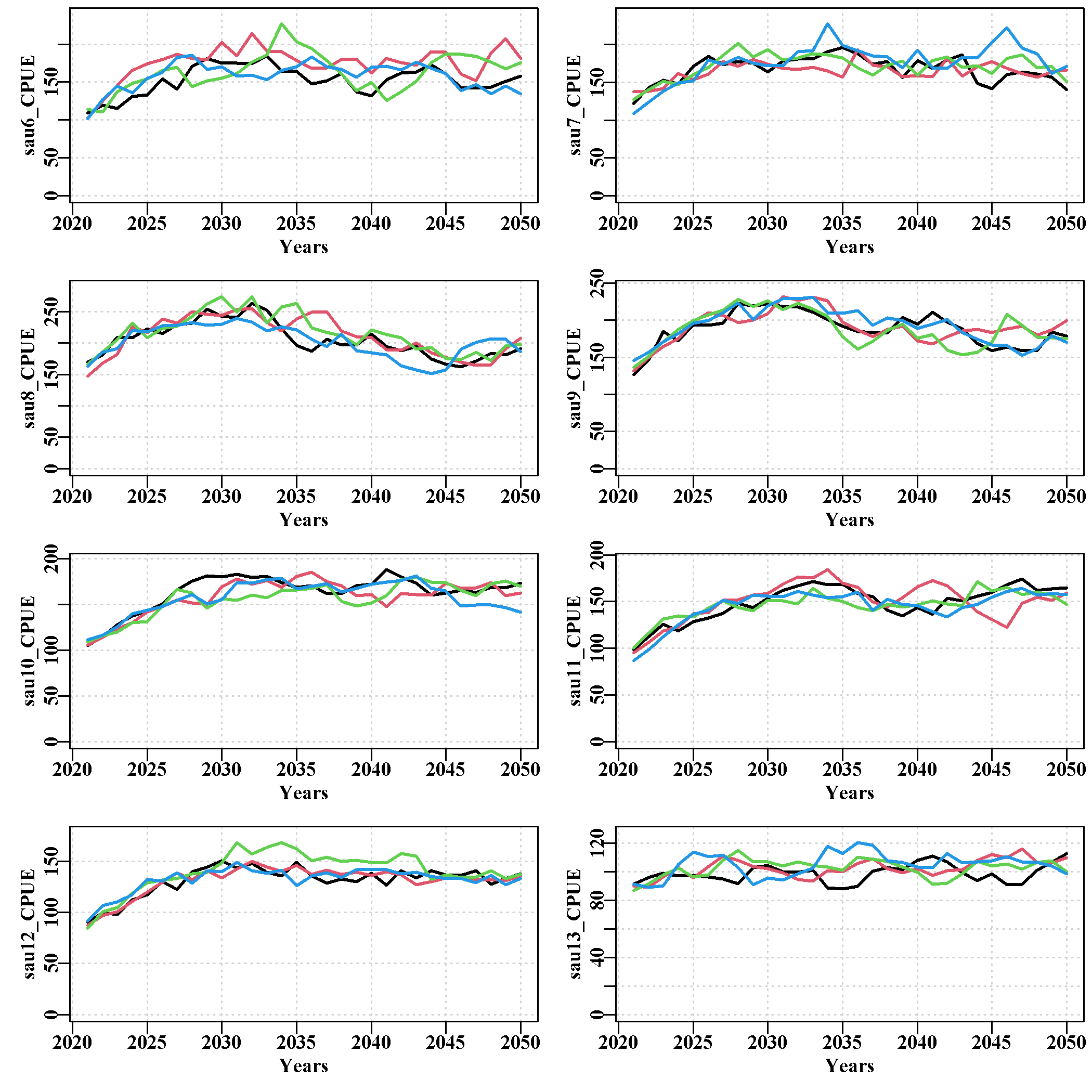
3.5.16 DiagProj Page
Currently contains three plots designed to characterize some of the variability of the projections and to ensure that the expected dynamics are behaving in a manner akin to the real fishery.
The first plot is of the differences between the actual SAU catches and the aspiration SAU catches, while useful this plot needs improvement to denote the proportional error in each SAU. Within the current Tasmanian HS when actual catches begin to approach 120 percent of the aspirational catch then that sau is closed to further commercial fishing. The 120% value has been reduced in recent years, meaning the withsigB value needs to be reduced. This acts to limit the variation now possible. This can be used to ‘tune’ the withsigB value that is used to control how precisely the fleet dynamics adheres to the aspirational catches derived from the harvest strategy. If withsigB was set extremely small, then the variation included in how much catch was taken from each sau and each population would also be small. The calcpopC() function, which estimated the aspirational catches (and TAC) is defined in EGHS (or whichever harvest strategy is being used). The algorithm underlying the dynamics is described and explained in the documentation to EGHS (and hopefully in any other HS as well). The fleet dynamics essentially describes how the divers interact with the harvest strategy and hence needs to be part of the input functions as part of the HS package or R source file.
The second plot is a comparison of a limited number of randomly selected trajectories from the scenario being explored showing the actual catches by SAU, as solid lines, and the related aspirational catches as dotted lines. This plot functions to show that the fleet dynamics model is behaving in a realistic manner but also to illustrate whether the expected variation in catches by sau are plausibly realistic. In fact, they are far less variable than during the history of the fishery (see the fishery tab) but this is a reflection of the meta-rules that control the deviation from the aspirational catches, that were only introduced in 2019. The number of lines plotted is determined by the ndiagprojs=4 argument within the do_MSE() functions argument list. With four lines, this is readable but if this is set too large the plot becomes too busy and loses any value for diagnostics, even when magnified.
The third and final plot is of the same number of individual CPUE trajectories for each sau. Again, its purpose is to determine whether the variation in the predicted CPUE trends appear realistic for the fishery concerned.
3.5.17 zonescale Page
Like the projSAU page, this contains seven plots of the same set of plots as seen in the projSAU page, but of zone scale dynamics. The projected values for each population within each SAU have all been combined at the zone scale (catch weighted where required, see the help for the function using ?poptozone). The plots include total catch, the TAC (essentially the same plots in Tasmania), CPUE, and mature biomass depletion level, mature biomass (mirrors the depletion plot), annual harvest rate, and annual recruitment.
Of course, the zone scale dynamics obscure the variation observed at the SAU level and even more so at the population level. The zone scale ultimately, is of principal interest in terms of the consequences of a particular HS scenario for the TACC, while the SAU and population scale details provide an understanding of the spatial complexity within the zone and the relative reliance on the different SAUs.
The page ends with a table containing the median values of each of the plotted variables.
3.5.18 Fishery Page
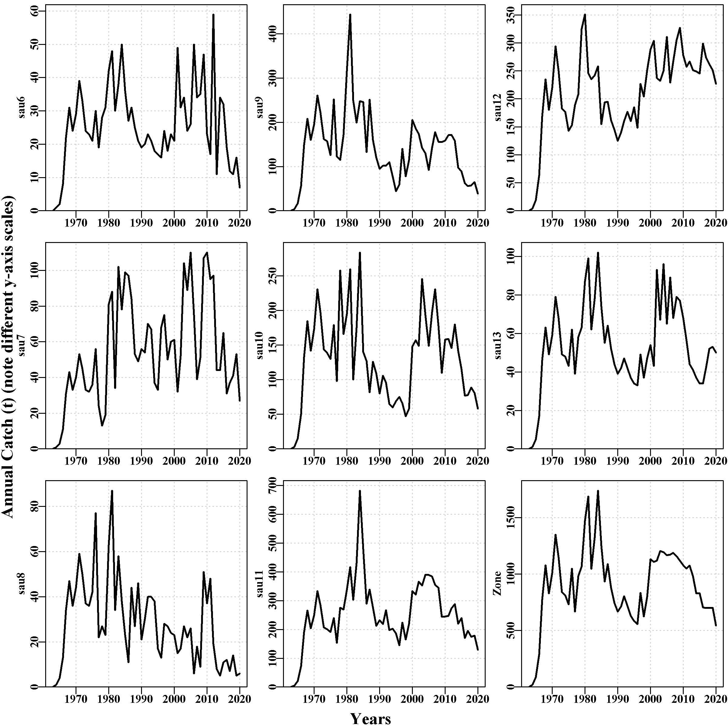
This page was intended to illustrate the historical fishery data. It currently contains a plot of the selectivity curves relating to all LML that occurred during the historical conditioning period and through the projection period. Then a plot of the individual catches by sau, which illustrates the remarkable inter-annual variation in historical catches in teh Tasmanian western zone blacklip fishery. Some sau exhibit halving and doubling of catches in the space of two years. Even the final zone-wide sub-plot exhibits some large changes between years, although this calmed down a good deal at least at the zone scale once quota zones were introduced in 2000.
The final plot is of the cpue observed in each sau. Note the truncation of the time-series in sau6 and sau13, which occurs because the introduction of zonation in the year 2000 split these sau across different zones.
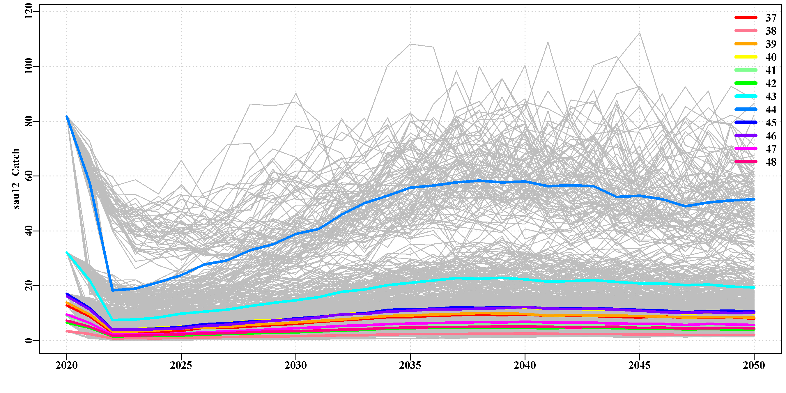
3.5.19 HSperf Page
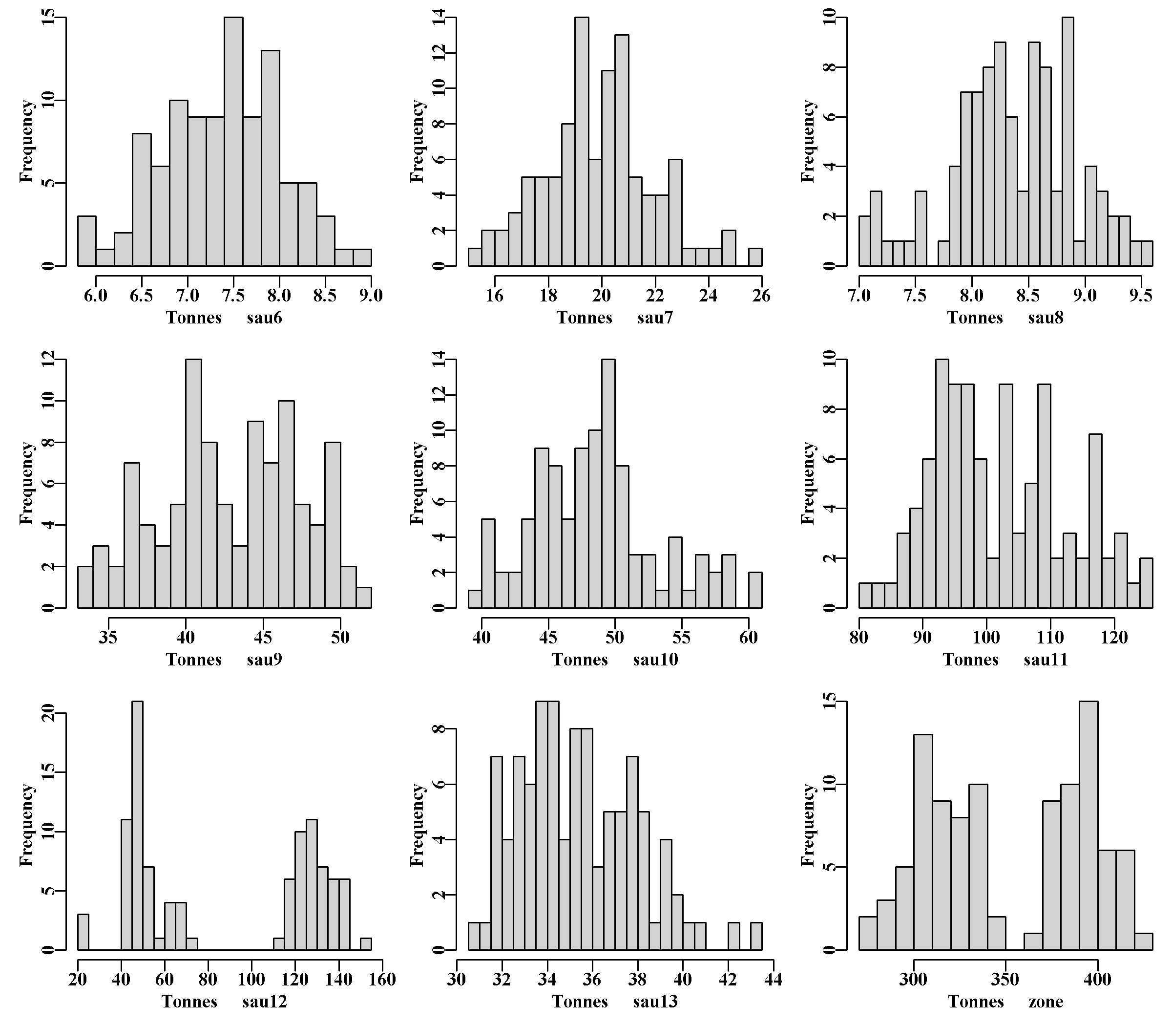
This page currently holds a listing of the arguments used by the harvest strategy (hsargs) and plots of the cumulative sum of total catches by sau at 5-years and at 10-years as well as plots of the mean catches at 5 and 10 years, again by sau. The hsargs listing is simply a double check that the values used are what was wanted.
The bi-modal outcome for sau12 is obvious and appears to relate to some random recruitment events leading to lower biomass and CPUE, and in some cases an aCatch reduction of 75% or even two such reductions. The final table is an example from a single replicate of what target cpue is achieved through the projections for each sau. It is the case that sau6 to sau10 invariably breach the 150kg/hr imposed maximum, while sau11 - sau13 all achieve a somewhat lower target, with the more easterly sau having lower targets.
It is expected that these tables and plots will differ for each harvest strategy examined.
3.5.20 scores
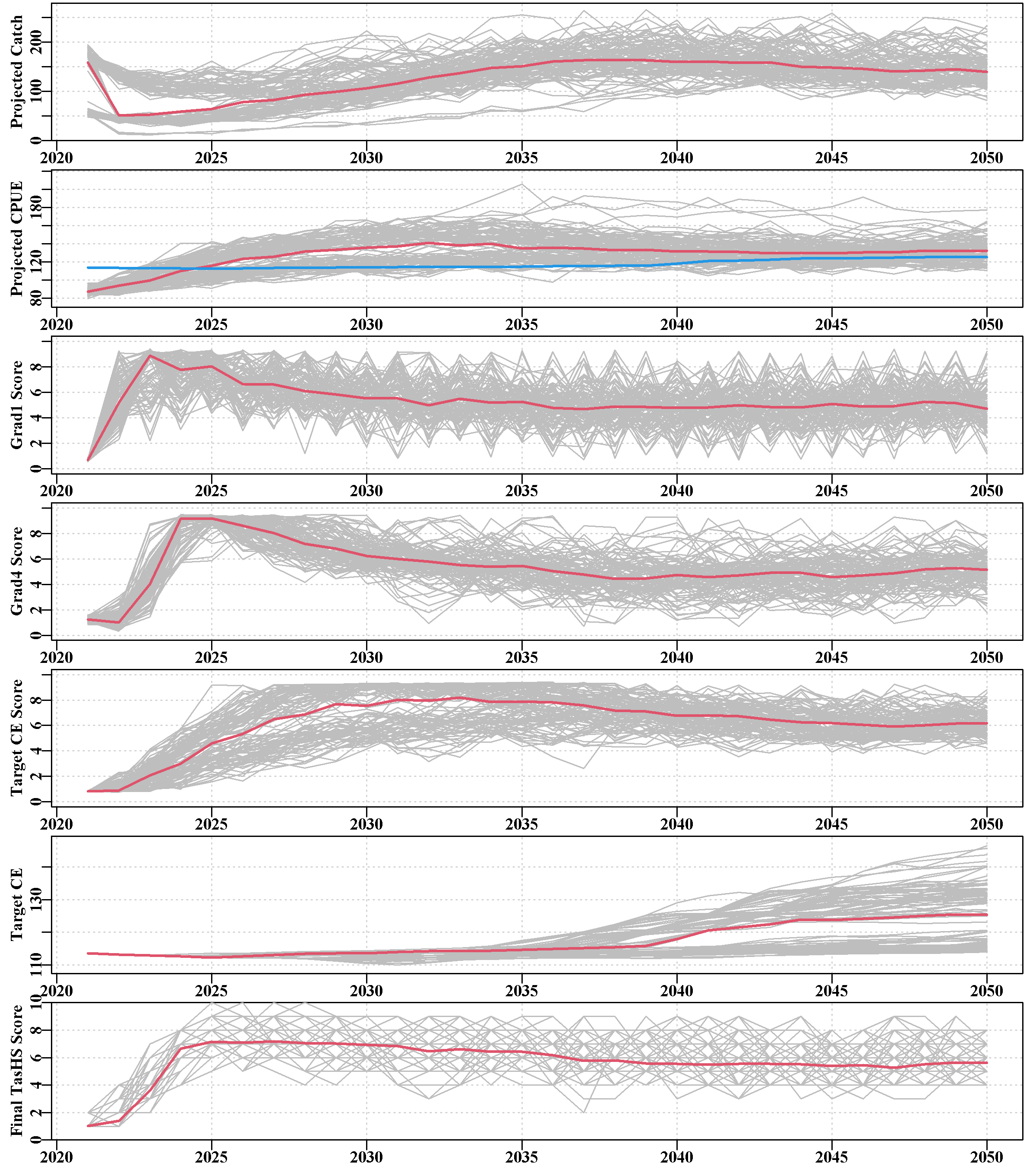
The scores page illustrates the HS statistics for each sau. Each plot depicts the projected catch and cpue, and the scores for the grad1, grad4, and targetCPUE performance measures (PM). Finally, it provides the targetCPUE and the final total score from the harvest control rule.
These plots enable the user to determine which fishery PM contributed most influence on the catches and when.
The red lines, in each case are the median values.
Once again, the illustrated plots relate to the Tasmanian harvest strategy and its variants. Differing plots will be required to be relevant for different jurisdictions. Equally, the interpretation of any resulting patterns will be dependent on the jurisdiction’s HS. For example, in Tasmania, the median final TasHS score is expected to stabilize at 6, which is the index of the multiplier = 1.0 in the hcr argument of Tasmania’s hsargs.
3.5.21 poplevelplots
Each sau has a given number of ‘areas of persistent production’ or populations. This tab on the website contains plots of the replicate trajectories within each such population within each sau. The median value for each population is also plotted as a unique colour. Such population level plots illustrate the degree of heterogeneity in productivity between the populations within each sau.
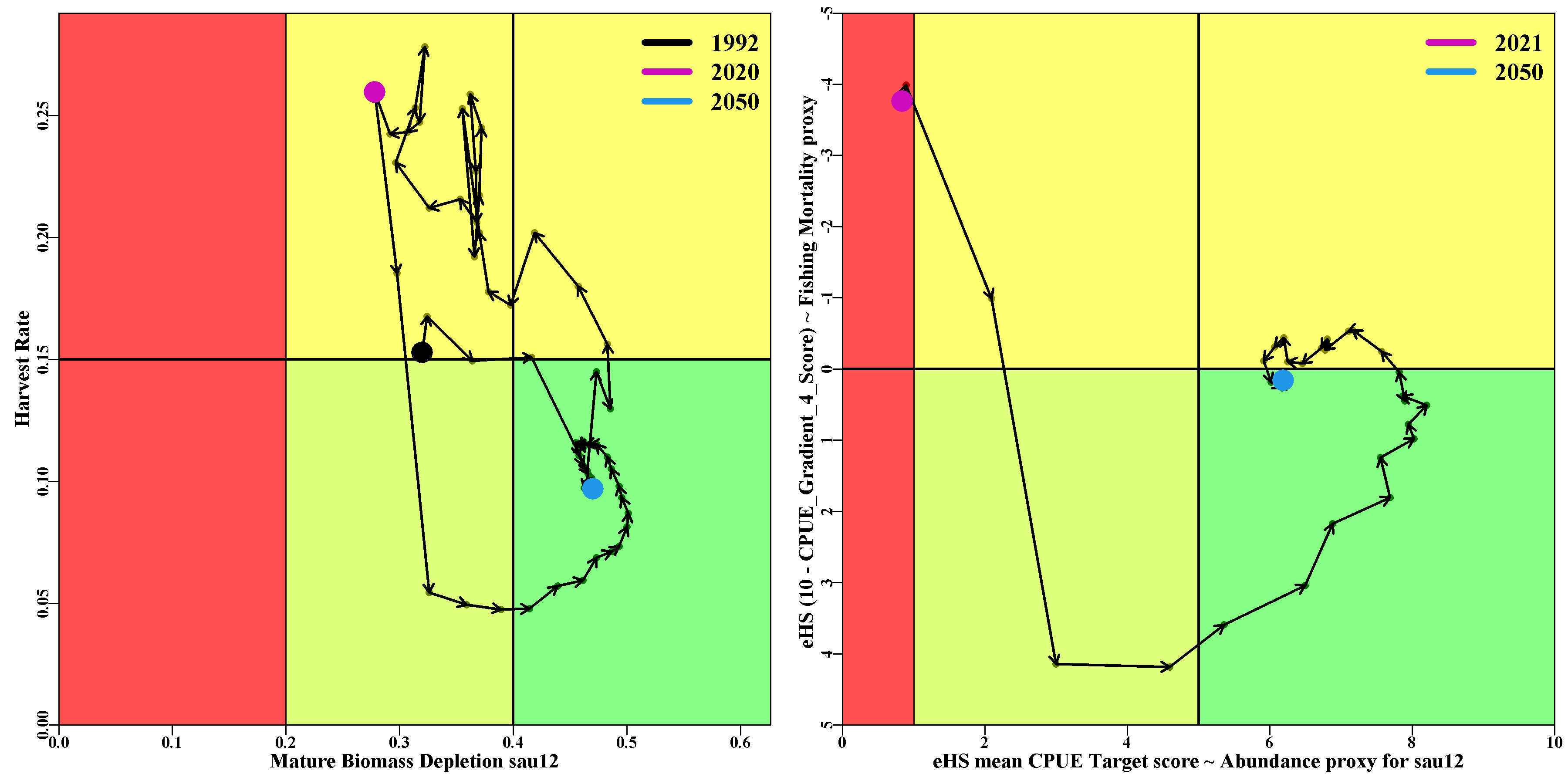
3.5.22 phaseplot
The phaseplot tab contains eponymous plots for each sau. For each sau there are two phase plots (or Kobe plots if you will). The first is a more classical plot of the predicted Harvest Rate vs the predicted Mature Biomass Depletion level and contains all the data from the start of the CPUE time-series to the end of the projection (the projected parts use the median, although this may evolve to show some possible bounds). The second plot is of the CPUE gradient-4 score from the EGHS vs the CPUE Target score from EGHS. The first is to act as a proxy for the fishing mortality or harvest rate, and the CPUE target score acts as a proxy for the mature biomass. The two plots for each sau are placed side by side to make comparisons between the theoretical optimum variables and their proxies (which do surprisingly well).
A table is provided containing the final values (2050) for each SAU, of the metrics used in the phaseplots.