| sau | pop | AvRec | L50Mat | SaMa | DLMax | L50 | L50inc |
|---|---|---|---|---|---|---|---|
| 5 | 1 | 0.1 | 99.5 | -15.969 | 21.8 | 112 | 31.5 |
| 5 | 2 | 0.4 | 98.9 | -15.969 | 24.0 | 112 | 38.5 |
| 5 | 3 | 0.1 | 113.0 | -25.853 | 26.6 | 115 | 34.9 |
| 5 | 4 | 0.4 | 115.0 | -25.853 | 22.6 | 115 | 40.1 |
8 Conditioning by Population
8.1 Summary
The AIRF project 2023_63 has enabled the aMSE code base developed during the FRDC project 2019-118 to be expanded to allow for population-based conditioning of individual populations within different spatial assessment units (SAU). The option of population conditioning is now available although if is not used it has no effect on the simulation outputs. Population based conditioning is required when attempting to answer tactical issues such as the effect of making a change to the legal minimum length (LML) in areas where the heterogeneity of productivity is very great (such variation is common in blacklip abalone stocks). In addition to adding these new options, an array of new outputs relating to population-based dynamics and properties have also been implemented, which, again, are designed to facilitate answering SAU specific questions relating to optimizing management decisions other than catch levels. All of these changes now operate seamlessly within the codebase.
8.2 Introduction
In previous sections, methods for conditioning the operating model within the MSE have been described. Assuming it has been possible to use the sizemod package to fit to data from each SAU, ideally, the dynamics of each SAU, as they are predicted by the aMSE software, should be very similar to that expressed by the individual SAU in the sizemod software. Differences can be expected because in the aMSE package each SAU, instead of being treated as a single dynamic pool population (as it is in sizemod), is represented as a set of mostly separate populations.
Prior to the changes described in this chapter the biological properties of each population within each SAU are based upon the properties expressed at the SAU scale, albeit with random variation included on almost all biological properties. The degree of variation added in the examples is set to a level in each case to mimic the spatial heterogeneity in productivity typically expressed by the blacklip abalone around Tasmania). When conditioning by SAU the current property that is an exception to this strategy is the average unfished recruitment level (R0 or AvRec), estimated as a parameter for each SAU by sizemod. Now, in aMSE, the SAU level AvRec is sub-divided across each SAU’s populations on a fixed proportional basis, which will be unique to each SAU (and has been derived from the relative yield from the population areas as defined using the GPS logger data). The method of implementation can be seen in the Chapter 5 under the propREC section. As a result of this variation, there can be many differences between and within SAU and how they are represented in the MSE.
The development of both the aMSE and sizemod R packages was partly driven by needing to solve the various problems associated with providing a generalized framework for conducting MSE analyses on spatially structured benthic fisheries on species that required size-structured dynamics (because they were hard to age). The sizemod R package was developed as a means of conditioning the MSE operating model within aMSE such that its predicted dynamics attempted to match both the observed CPUE as well as the observed size-composition of the catch of abalone. The advent of sizemod led, in turn, to improvements to aMSE because of the new options presented by the outputs of sizemod. It is still the case, however, that some of the outputs from sizemod need to be modified slightly when they are represented by multiple populations within each SAU.
In some parts of the fishery more information is available concerning some aspects of the biology such as the size-at-maturity and growth. There are sometimes large differences in yield between some areas of persistent production (app or population), which are not able to be accounted for merely by including random variation and modifying the average unfished recruitment (AvRec) for a particular app/population. In addition, it can sometimes be desirable to set up scenarios where groups of apps within SAU have either low, middling, or relatively high productivity. In such cases some way of manipulating the variables important to productivity within individual apps (=populations) is required. The proportional strategy used to allocate unfished recruitment across the collection of apps within each SAU is not suitable for fixing values of size-at-maturity or growth in particular populations, so an alternative approach was developed and implemented.
8.2.1 Variables Important for Productivity and Yield
A number of model parameters relating to biological properties important for productivity exist. These include:
- average unfished recruitment, AvRec
- the growth parameters, here we use the maximum growth increment, DLMax, and the length at 5 percent of the maximum increment, L95 (= L50 + L50inc)
- the size-at-maturity, here we use the L50mat parameter (= length at 50 percent maturity) and the SaMa, or size-at-maturity ‘a’ parameter, the intercept of the maturity ogive with length
- the instantaneous natural mortality rate, M
- the steepness of the stock recruitment relationship, h (from the Beverton-Holt stock recruitment curve)
- the weight-at-length relationship, here we use the exponential b parameter of the \(W_L=aL^b\) that represents the weight at a given length \(W_L\).
How these can be allocated individually to particular populations/apps is the subject of this chapter.
8.2.2 The Difference between Productivity and Yield
The notions of productivity and yield sometimes appear confounded in the fisheries literature but their differences are clear.
The yield from any area is simply the amount of catch that has been removed over whichever time-frame is being considered. Whether the ‘yield’ should include any other fishing related mortality is a complication best avoided by treating that separately. With abalone, non-fishing related mortality should be minimal, especially as when divers accidentally remove sub-legal sized animals from the rock, they are required to place the animals back on a rock surface and ensure they adhere. Illegal, unreported, and unregulated catches (IUU catches), such as that due to poaching or even recreational fishing, should be treated separately where there is available information.
Productivity is a more complex concept than simple yield. It relates to the rate of production of potential yield, which is one reason the two concepts can get confused. For example, the somatic growth of individuals is a strong contributor to a population’s productivity. Thus, a low productivity reef of the same area as a higher productivity reef will, on average, produce a lower yield because the individuals in the more productive population are expected to grow past the legal minimum length (LML) faster and to grow to a larger, heavier size. Two equal sized reefs might produce the same yield in a given year, but the more productive reef will be able to sustain such catches for longer. Generally, a lower productivity area would be expected to have slower growth, a smaller maximum size, and possibly a lower size-at-maturity. The possible yield is determined both by the biological productivity and the legal minimum size, as well as the area of a reef. A key factor for abalone sustainability is setting the legal minimum size appropriately.
The caveat above about ‘same size reef’ is important, because, in principle, it would not be impossible to obtain a seemingly high yield from a relatively low productivity area if that area was large. Even so, it would not be expected to be able to sustain large catches for as long as an equivalent high productivity area. Similarly, if the available reef area of a highly productive population was low then the potential yield from it will also be low. Despite this, a difference between the two is that it is easier to deplete a higher productivity area if the legal minimum size is set at a size that enables the fishery to deplete the spawning biomass. If the LML is set at a size that allows good access to slower growing, less productive populations in an SAU (spatial assessment unit), this will increase the risk of over-fishing for faster growing, more productive areas, which, very sensibly, are generally preferred by divers.
As natural mortality is generally strongly related to somatic growth rates and maturity, natural mortality is also expected to be strongly influential on productivity (Beverton, 1992; Jensen, 1996). However, as is typical in most fisheries, estimates of natural mortality for any species are generally poorly defined, and this is especially the case with species that are difficult to age. Abalone around Tasmania appear able to live to at least 30 years of age (based on growth rates and maximum sizes), which using simple life-history relationships implies a natural mortality rate of about 0.15. This is generally used along with slight variation among populations. When attempting to adjust the productivity of individual populations (=apps) it is recommended that changes be made to growth, maturity, and recruitment, rather than to natural mortality.
The average long term yield from an area is correlated with the area of reef fished (determined using the combined areas of the KUD derived from the GPS logger data). So, when attempting to set the productivity AvRec, or the proportion of recruitment allocated to a population, should perhaps be the first variable to modify. The total AvRec influences the SAU’s total population, so changing that will alter each population according to its allocated share.
After having set up the SAU approximately to the level reflecting that observed in the fishery, it is recommended that when proceeding to condition on individual populations then the parameters on which to concentrate relate to somatic growth and maturity. Of course, if required, any of the model’s parameters can be added to the list of those fixed by population. For example, the steepness (defsteep) in the data file) can be influential because it also affects the stock recruitment curve, although once the other parameters are fixed the effects of steepness become relatively minor.
8.3 Methods
A description of conditioning each SAU might summarize earlier sections by describing how a base case set of constants for natural mortality, steepness, and cpue hyperstability, lambda, were chosen for implementation within aMSE. Once selected, the available fishery and biological data for each SAU could be put through sizemod and the model fitted in a manner that estimated some growth parameters, the unfished average recruitment, and the average diver selectivity across sizes of abalone. In addition, sizemod estimates recruitment deviates across those years where sufficient size-composition data exist to inform the model. Other constants, such as those describing the weight-at-length are estimated outside of the model.
8.3.1 Relative Weighting of Data Sets
Within sizemod the relative weight attributed to the cpue index of relative abundance is described by Francis (2011; the so-called Francis weighting). At the same time, an iterative re-weighting routine is used to discover the optimum weighting to apply to the size-composition data. Finally, relative bias ramps are applied to the recruitment deviates to account for the varying amount of information available at the limits of the observed size-composition data (Method & Taylor, 2011).
Routines have now been developed that collect together the final optimum parameters into a matrix and these can now be automatically transferred to the control and data files used by aMSE so that the latest estimates of the important productivity parameters are easily transferred accurately from sizemod. To enhance comparability between the outputs of both sizemod and aMSE it is important that the assumed constants for such things as the weight-at-length, maturity-at-length, growth and all the rest are the same for each SAU in both software systems.
After transferring the parameters from the sizemod estimates into each SAU within the aMSE operating model further adjustments are required to the AvRec and recruitment deviates to optimize the fits between the predicted CPUE at the SAU level and the observed standardized CPUE as well as optimizing the fits between the predicted size-composition of catch and those observed. This is done within aMSE using the two functions adjustavrec() and optimizerecdevs() (see their individual help pages within aMSE for their arguments and the syntax for how to use them.
The differences between the predicted MSY and AvRec for sizemod and aMSE is such that for each SAU in the Tasmanian western zone the MSY in aMSE is about 9.5% less than the sizemod estimate for each SAU, and the AvRec is about 3.8% larger in aMSE, although that relationship is much more variable between SAU. These differences between the sizemod and the aMSE values are a result of the dynamics in aMSE being split between each SAU’s populations rather than a single dynamic-pool within each SAU SAU and the scale of the differences alters with the number of populations used within an SAU.
8.3.2 Conditioning the Operating Model at a Population Level
Much of the data used to condition the operating model is contained within the ‘saudataXXX.csv’ file (see Chapter 5 for a detailed description of the contents of each input file). Each SAU has a particular average value of the important variables to be set, such as DLMax and L50mat. In addition, there is an associated variability sDLMax and sL50mat used to define the variation used when randomly varying each parameter across the populations within each SAU. For what follows it is important that the name of the variation parameter is identical to the variable it relates to except for the prefix ‘s’. This is because the names are used explicitly when identifying which parameters are to be set by population and which are to remain randomly allocated across populations. Those that are to be set by population need to have their associated variation set to a very small number (e.g. 1e-06 or smaller) so that when variation is added it does not affect the set value.
8.3.3 An Hypothetical Example
An hypothetical sauX can be used to illustrate what changes are required to implement population-based parameter setting. The example will be unrealistic as only four populations will be implemented within a single SAU so that the example is simple to follow (a matrix of four rows is easier to follow than one of 30 rows). In real simulations there would generally be many more separate populations. For example, the western zone simulation used in FRDC project 2019-118 had 56 populations across the eight SAU. When conditioning by population the potential to increase the spatial detail is greater.
We are using the catch, cpue, and size-composition data from sau5 in Tasmania’s Northern zone to form the basis of our hypothetical SAU. In reality, the number of identifiable populations within sau5 is somewhere between 13 and 24, with a final number to be decided through consultation with experienced industry members regarding on-the-ground fishing behaviour.
The structure and contents of the control, data, and size-composition data files are described in the chapter on The Input Files (Chapter 5). No changes are required to the control file. The bysau flag, under the START section in the control file should remain set = 1:
- START,,,,
- runlabel, sauX , the scenario label,,
- datafile, saudatasauX_by_sau.csv , name of saudata file,,
- bysau,1, 1=TRUE and 0=FALSE,,
- …
Prior to AIRF project 2023_63 the bysau flag was inserted into the code base in readiness in case an opportunity came to condition the population properties directly rather than as random variation from SAU properties. Once starting the 2023_63 project, after some false starts, it soon became clear that there was a more effective way of implementing population-based conditioning that did not need the bysau flag. Rather than produce a large and difficult to use matrix of all variables (minus the variation terms) by all populations it is much more efficient to only modify those variables that influence productivity (or other aspects of the fishery that are to be explored) and leave the rest as random variation from SAU averages. The bysau flag is now deprecated and eventually it will be removed from the code. It is retained in the meantime to avoid the potential for disruption of other users of the aMSE software. If the flag is set to its default value of 1 (as in: bysau, 1,) then the flag will continue to have no effect on any of the scenarios.
Instead of using the bysau flag a simpler solution for the user was to allow the software to determine which parameters were to be fixed for each population when reading in the data file. This is the source of the requirement that care is needed when typing the names of the selected parameters. When no population conditioning is used, which was the only option developed prior to AIRF project 2023_63, the propREC section only referred to the proportion of each SAU’s AvRec (average unfished recruitment level) allocated to each population. Obviously, the proportions across all populations sums to 1.0. In the data file this is represented using the following lines at the bottom of the file (see Chapter 5; the symbols at the start of each line in the text are not included in the data files):
- propREC,,
- sau, pop,AvRec,
- 5, 1, 0.1,
- 5, 2 ,0.4,
- 5, 3, 0.1,
- 5, 4, 0.4,
In the single-SAU-four-population example of sauX we will illustrate fixing the L50Mat, the size at 50% maturity, SaMa, the intercept of the maturity ogive , DLMax, the maximum growth increment, L50, the size at half the maximum growth increment, and L50inc, which is used to produce the L95 growth parameter (\(L_{95}=L_{50} + L_{50inc}\)).
When implementing population-based conditioning, where selected variable/parameter values are defined or fixed in each population, it is necessary to provide values for each of the selected parameters for each population implemented in the operating model. The implementation involves expanding the original propREC section at the bottom of the data file. Perhaps the section should no longer be termed propREC, but again, to prevent disruption to other users this name will be retained (for the time being; naming things when writing software is harder than it might look).
The names used in the first line below the propREC label must have exactly the same spelling and capitalization as is used in the table of SAU parameters that make up the top of the data file (see Chapter 5). The first three columns remain identical to the default conditioning setup (as above). We have added the five parameter names and the respective values that we wish to allocate to each of the four populations.
In the north-west for example, we might use an analysis of the extensive data set available on the size-at-maturity across sau 5 and 6 to define a more specific set of values for the different populations identifiable using the GPS logger data. Similarly, in consultation with Industry divers, the relative productivity expected from each smaller area within each SAU can be used to select appropriate values for the growth parameters. Such conditioning at a finer geographical scale than the SAU is very dependent upon the GPS logger data. But this finer scale is required to make sense of the heterogeneity in productivity expressed by the various areas of persistent productivity identified within the north-west.
The data file, with most unchanged lines omitted, should now have the following form:
- Biological properties by population for hypothetical sauX
- SPATIAL,,
- nsau,1, number of spatial management units
- saupop,4, number of populations per SAU in sequence
- saunames,X, labels for each SAU
- PDFs,32,
- DLMax ,23.50603217, maximum growth increment
- sDLMax ,1.00E-06, variation of MaxDL NOTE tiny value
- L50 ,112, Length at 50% MaxDL
- sL50 ,1.00E-06, variation of L50 NOTE tiny value
- L50inc ,30.34957282, L95 - L50 = delta =L50inc
- sL50inc ,1.00E-06, variation of L50inc NOTE tiny value
- …
- AvRec,878733.028324352,
- sAvRec ,1.00E-07, NOTE tiny value
- …
- SaMa,-22.371, maturity logistic a par
- L50Mat,98.8992042, L50 for maturity b = -1/L50
- sL50Mat,1.00E-07, NOTE tiny value
- …
- propREC,,
- sau, pop,AvRec,L50Mat,SaMa,DLMax,L50,L50inc,
- 5,1,0.1, 99.5,-15.969,21.8,112,31.5,
- 5,2,0.4, 98.9,-15.969,24.0,112,38.5,
- 5,3,0.1,113.0,-25.853,26.6,115,34.9,
- 5,4,0.4,115.0,-25.853,22.6,115,40.1,
Note the single-sau-four-population spatial structure under SPATIAL. Each of the five parameters fixed to population specific values has its related variation value denoted with the same name prefixed with s, as, for example, sDLMax and sL50inc. The SaMa parameter does not have additional variation as the weight-at-length relationship it affects is extremely sensitive to this value and adding even small amounts of variation led to unpredictable outcomes. In each case these sParName values have been set to very low value such as 1e-06 or 0.000001. When each population is generated within the aMSE software, including this much variation leads to no noticeable change to the fixed values.
If the user forgets to set the variation variable to a very low value and yet sets up the rest of the data file to fix specific parameters, then a warning message is generated. Similarly, if a parameter is not set up to be fixed for each population but the variation term is still set very low, a different warning message is generated.
8.3.4 Other Details
Earlier data files were somewhat odd in that the variation term for the DLMax was named sMaxDL.
- PDFs,32,
- DLMax, 23.50603217, maximum growth increment
- sMaxDL, 1.00E-06, MaxDL name decremented, replaced by sDLMax
- L50, 112, Length at 50% MaxDL
- …
This is merely an historical hang-over, which once started was hard to change without bothering all current users of the program. Fortunately, an approach to fixing this has now been developed. Should a user begin developing a scenario using this older format the software will automatically rename the sMaxDL as sDLMax in the ‘saudata.csv’ file to allow correct usage of population-based conditioning, and it also issues a warning pointing out that sMaxDL is deprecated and has been changed. The end result is that users can continue to use older data files without issues arising. This strategy may be applicable to other deprecated instances that have developed from the on-going implementation of expanded options within aMSE.
8.3.5 Other Code Base Changes
With the advent of population level conditioning some novel model output relating to the population scale have now been included in the standard aMSE output. These will enable the individual dynamics within each population to be visualized and examined in more detail. This will be of great value if, for instance, an investigation was made of the implications of changing the Legal minimum length in SAU’s that have populations that exhibit large differences in growth and productivity (as is now happening in Tasmania’s NorthWest).
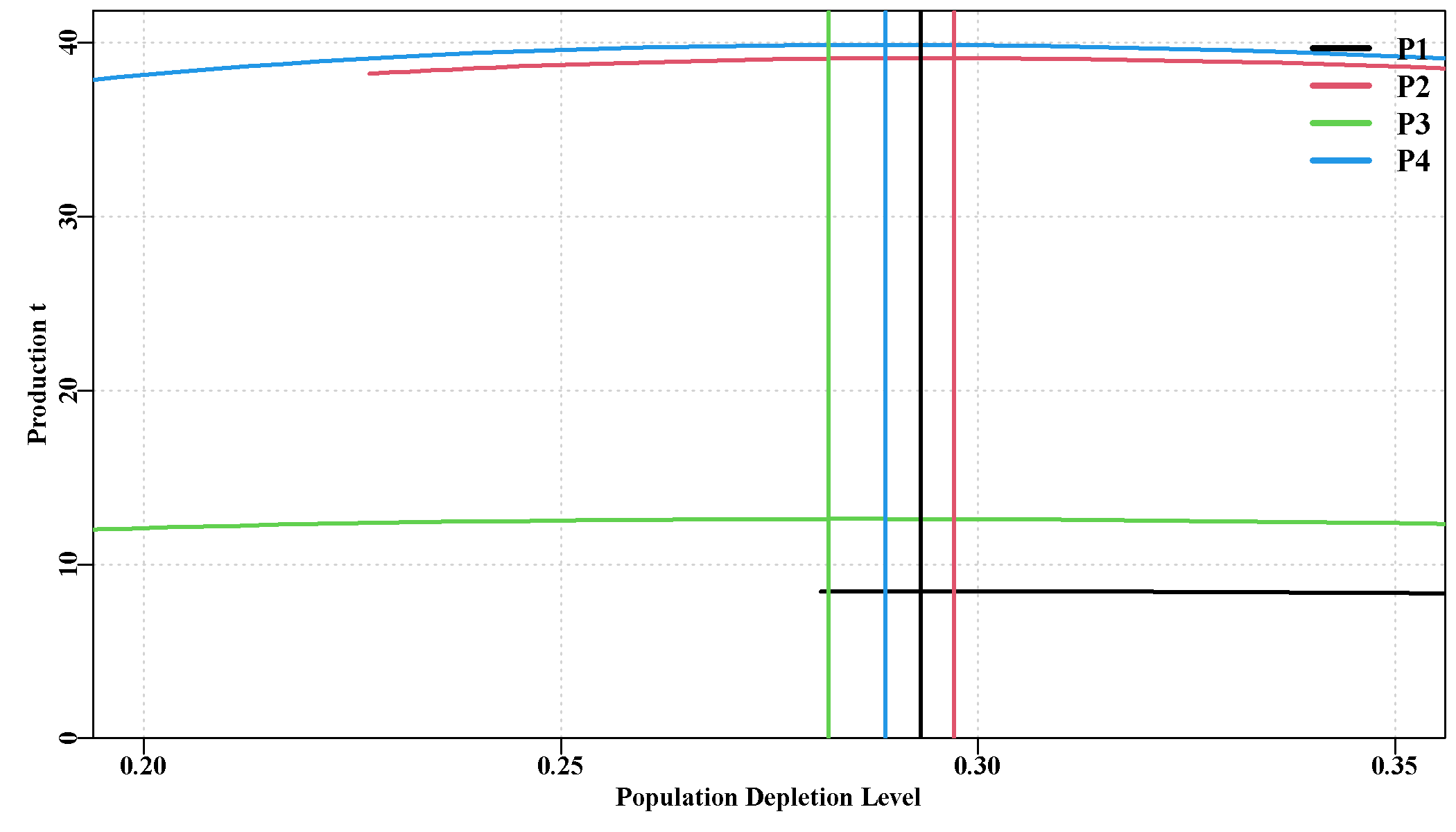
Some of these additions are illustrated below from the sauX example, the four populations were set up to have approximately two different levels of productivity.
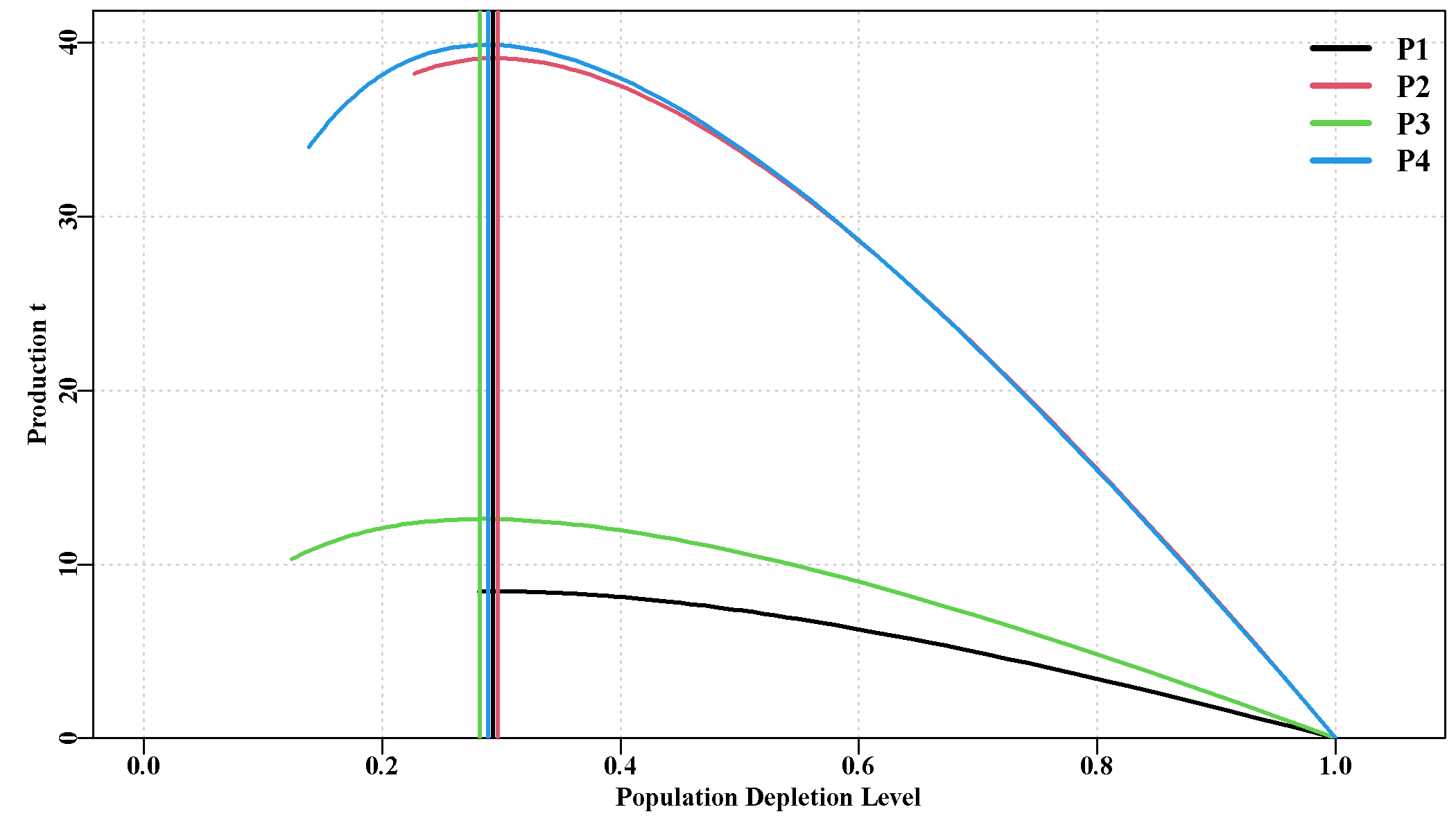
Note how in Figure 8.1 all four populations have their maximum productivity at very similar spawning biomass depletion levels despite having very different productivity. In fact, the production is relatively flat between depletion levels of about 25 - 35 %
Numerous other small but important changes were required in many places throughout the aMSE codebase once the population-based conditioning was implemented to ensure that the most recent changes do not alter the functionality of the software when population conditioning is not used.