6 Conditioning the MSE with the sizemod Package
6.1 Introduction
A Management Strategy Evaluation can attempt to simulate a real-world fishery. Conditioning the operating model involves modelling the properties of the fished stock so that the dynamic behaviour of the operating model mimics, or is at least has strong similarities to, the observed dynamics of the real-world fishery. Where operating models assume no or only simple spatial structure, it is sometimes possible to use standard stock assessment modelling methods to fit the operating model to available data from the fishery. This would ensure that estimates of productivity and other aspects of how the stock responds to fishing pressure are as good as the available data permits. Fitting the operating model to available data would also provide estimates of uncertainty around key parameters, which could then be included in the MSE simulations to provide a relatively realistic reflection of how the stock could respond when using alternative harvest strategies to provide management advice through time.
In Australia (and elsewhere) abalone stocks tend to be made up of meta-populations with notoriously complex spatially structures, with each component population being mostly self-sustaining through localized recruitment processes meaning limited larval movement and with very limited to no effective movement of settled animals. One outcome of such spatial structure is that most abalone populations can be considered data-poor (Haddon et al., 2005; Orensanz et al., 2005; Parma et al., 2003). Parma et al. (2003) and Orensanz et al. (2005) discuss the notion of S-fisheries, which are generally spatially structured (meaning patchy with heterogeneous biological properties), often targeting species of lower economic importance, and potentially subject to serial depletion. Wilson et al, (2013) added to this list of properties, by referring to the common mismatch between scale of fishing, scale of reporting, and scale of management (lots of S’s, hence S-fisheries). Most importantly, for this discussion, such fisheries do not conform to the assumptions of the classical dynamic-pool notion of fish stocks. For a fishery to be a dynamic pool then some population event (be it a fishing event, a recruitment event, etc) will affect the whole stock within a relatively short period (often, at most, within a year). This requires there to be relatively high levels of mobility and mixing of individuals, or at least high levels of larval movement. Such an assumption may well be valid in scale-fisheries but is far less often true in fisheries for sessile, sub-tidal, hand-gathered species. Abalone cannot be considered to be of lower economic value but closely meet every other criterion for S-fisheries.
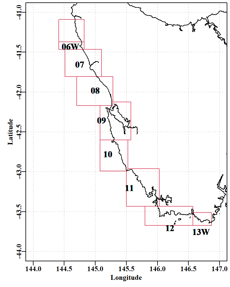
Given the complex spatial structured exhibited by Australian abalone fisheries it would be invalid to attempt a zone-wide assessment of a fishery’s dynamics and expect such a thing to reflect the observed dynamics at smaller geographical scales. At best, it might be possible to conduct an assessment at the smallest spatial scale at which data from the fishery has been reliably collected. In the case of the Tasmanian west coast, that scale is that the level of statistical block (= sau or SAU).
Generally, high value species around the world are assessed using relatively complex stock assessment models with statistical integrated assessment models becoming more common (Maunder and Punt, 2013; Punt et al., 2013). High value species such as abalone are not often considered to be data-poor species, but there are many difficulties in collecting representative data from such a patchily distributed, highly variable, sub-tidal species. In the case of Tasmanian blacklip abalone (Haliotis rubra) data collection with respect to the biological properties of size-at-maturity, growth, and size-structure, has continued for decades. However, the extent and complexity of the Tasmanian coastline means that many areas and depths have no such biological samples at all. Spatial complexity and heterogeneity becomes a problem when attempting to condition the aMSE operating model to mimic the dynamics of an Australian abalone stock (see the appendix on Maturity vs Location for an example of small spatial scale biological heterogeneity).
6.1.1 What Models are Possible?
Surplus production models (Prager, 1994; Haddon, 2011, 2021) have been used with some success with catches and standardized CPUE data from some Tasmanian abalone statistical blocks. The SAU on the west coast with the most data (SAU 9 - 12) provided relatively convincing model fits to the available data. The sparser data from SAU 6 - 8 generated less stable model fits, mainly because catches, and therefore number of records, were relatively low and the limited data were therefore more variable. The original idea for conditioning the Tasmanian MSE was to use such models to estimate the productivity of each block/SAU and continue improving the fit to observations from there. One problem with this strategy is that simple surplus production models assume that recruitment is also a simple and deterministic process. Unfortunately for this strategy, in Tasmania, abalone recruitment is sometimes extensive and far from average across whole quota zones and at other times appears patchy and variable in intensity. In the operating model, annual recruitment is modelled using a Beverton-Holt stock recruitment curve. Exploratory attempts to impose trial and error recruitment deviations from the modelled averages into the surplus production models, demonstrated that recruitment deviates were necessary for the predicted CPUE and predicted size-composition of the catch to approximate the observed data. However, attempting to introduce such artificial recruitment deviates was clumsy at best and often led to implausible model inputs at worst. Another disadvantage of using surplus production models is that they ignore what is known about the biological properties of the different areas (differing growth, etc.), and they cannot use any of the size-composition of catch data, which are now regularly collected, when fitting the model. These disadvantages are a problem because together they mean such models cannot provide strongly defensible estimates of any recruitment deviates that may have occurred.
Despite the serious issue regarding how representative of the multiple populations expected in any one SAU standard sampling can be, the use of a size-based integrated assessment model was explored to determine whether it could provide more plausible estimates of productivity and, more especially, of the expected recruitment dynamics during the known history of the fishery. An R package, called sizemod has been and continues to be developed to simplify the application of such a model; it is documented elsewhere and within the sizemod package. Here we will focus on different ways of using it and what the modelling results imply for conditioning aMSE’s operating model.
6.2 Using sizemod as a Size-Structured Production Model
The R package sizemod contains a number of data files that allow for the illustration of how to use the software. One data set, fish, contains the fishery data, another, sizecomp, contains observed size-composition data from catches across a number of years, and another setup contains other details required to get a model run to work (see sizemod documentation, which also contains a formal description of model structure.).
require(sizemod)
data(fish)
data(sizecomp)
fiscomp <- NULL
omega=c(1,1,0,0) # include data streams for cpue and size-composition, no FIS
data(setup)
ctrl <- setup$ctrl
glb <- setup$glb
constants <- setup$constants
glb$maxage=50
glb$phase=1
glb$lambda <- 0.75 # CPUE and Exploitable biomass relationship now non-linear
# when first fitting SA model set glb$sigce = 0, so between year CPUE
if (glb$sigce == 0) {   # variability is first approximated
  glb$sigce <- getrmse(fish,invar="cpue",inyr="year",natlog=TRUE)$rmse
}
biol <- makebiology(glb$midpts,constants) # define biological properties
kable(biol[50:59,],digits=c(3,3,3,3))| mature | WtL | emergent | MatWt | |
|---|---|---|---|---|
| 100 | 0.024 | 131.371 | 0.000 | 3.102 |
| 102 | 0.033 | 139.920 | 0.001 | 4.648 |
| 104 | 0.047 | 148.843 | 0.001 | 6.928 |
| 106 | 0.065 | 158.149 | 0.002 | 10.257 |
| 108 | 0.090 | 167.845 | 0.004 | 15.056 |
| 110 | 0.123 | 177.942 | 0.008 | 21.853 |
| 112 | 0.166 | 188.448 | 0.014 | 31.265 |
| 114 | 0.220 | 199.372 | 0.025 | 43.929 |
| 116 | 0.286 | 210.722 | 0.044 | 60.369 |
| 118 | 0.363 | 222.508 | 0.077 | 80.825 |
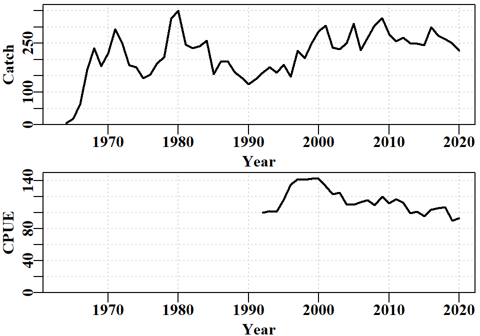
The catch time-series exhibits some remarkable variation from year to year (see Figure 6.2). The 100t increase between 1999 and 2001 in SAU12 was a response to the introduction of quota zones, which allocated a TAC to the west of Tasmania with the aim of distributing dive effort more widely around the State. The CPUE time-series only starts in 1992 because prior to that the data are an unknown mixture of records by month, day, individual diver, and collections of divers. A change in the reporting requirements in 1992 (daily by individual diver), and associated changes to the database helped solve those issues.
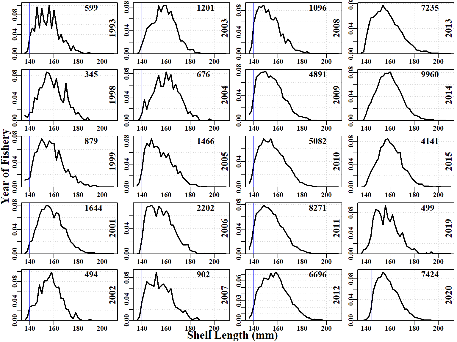
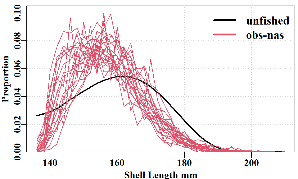
The size-composition data used was generally collected as samples of at least 100 individual measurements from individual landings by divers. Hence the early observations were often the outcome of sampling only very few landings. When combined with the 2mm size-classes in the assessment and operating models, this explains why the early data exhibits such spikiness. One great value of the size-composition data is that when it is compared with the theoretical unfished size-distribution of catches it provides a measure of the level of depletion imposed upon the populations within SAU 12. The size-composition data remains surprisingly noisy. For example, in 2019, the catches appear to be biased constistently high off the LML by about 5mm. Whether this was because divers had been instructed to try to ignore smaller animals for marketing reasons, or some other reason, is unknown. It suggests that time-blocking of any selectivity parameters might lead to improvements in model fit, although, once again, the question of whether the data are representative of an area as large as an SAU remains problematic (see Figure 6.1); the coastline of sau12 extends across about 0.4 of a degree of latitude and 0.5 degree of longitude.
6.2.1 The Initial Parameters
The model is currently set up to estimate about 35 parameters (depending on how many recruitment deviates are included), all of which are log-transformed to help stabilize the estimation process. These include the unfished recruitment (LnR0), the MaxDL of the inverse logistic growth curve used (Haddon et al, 2008), the L95 of the growth curve, the catchability (implemented to allow for a non-linear relationship between CPUE and exploitable biomass = hyperstability), and the difference between the 50% and 95% selectivity curve. In addition to these five primary parameters there are 30 recruitment deviates from 1985 - 2014. The number of deviates estimated depends upon the number of years of informative size-composition data there are available. Preliminary values for these are put into the model using a 35 x 2 array, with the second column containing a zero if the parameter is to be held constant and any number greater than zero (we use 1) if it is to be estimated by the model. By setting all the recruitment deviates to zero (back-transformed = 1.0), and setting the model not to estimate their value, it is possible to run sizemod as a size-structured surplus production model.
Difference in equilibrium population Numbers-at-size > 10 Difference in equilibrium population Numbers-at-size > 10 The initial parameters making up the pindat were obtained partly by examining the outcome of tagging estimates of growth in the area, and partly (mainly) by trial and error until the predicted CPUE at least approximated the shape of the observed CPUE (Figure 6.4).
6.2.2 The 5-Parameter Model Fit
By searching manually for initial parameters that provide an approximate solution, as suggested by the two curves approaching each other (Figure 6.4), then formally fitting the model to the available data becomes more efficient (see appendix for all the code used).
starttime <- Sys.time()
  outmod <- fitlbm(pindat,negLLP,funk=dynamics,biol=biol,glb=glb,fish=fish,
                   constants=constants,omega=omega,sizecomp=sizecomp,
                   fiscomp=fiscomp,both=TRUE,tol=1e-06,initH=0)
initial value 2565.279326 iter 10 value 1591.668939
iter 20 value 1527.720011
final value 1527.056570
converged
0: 1527.0566: 14.9410 3.16484 5.13042 -1.23772 -5.06285
Difference in equilibrium population Numbers-at-size > 10 fitpar <- outmod$ans2$par
optpar <- allpin
optpar[modin$notfix] <- fitpar
neglogL <- negLLP(pars=fitpar,initpar=optpar,funk=dynamics,biol=biol,glb=glb,
fish=fish,constants=constants,notfixed=modin$notfix,
omega=omega,finalcomp=sizecomp,fiscomp=fiscomp,full=TRUE)Difference in equilibrium population Numbers-at-size > 10 likelihoods <- cbind(oldlogL,neglogL,(abs(oldlogL - neglogL)))
print(round(likelihoods,4)) oldlogL neglogL
LLce 1163.1697 67.6058 1095.5638
compL 1401.0268 1457.8080 56.7812
penaltyR 0.0000 0.0000 0.0000
sigmaCE 0.0337 0.0337 0.0000
wtsc 0.0070 0.0070 0.0000
penLnR0 0.3574 0.9994 0.6420
penDL 0.0000 0.0370 0.0370
pencatch 0.0000 0.0000 0.0000
penH 0.7255 0.6053 0.1202
penaltyCE 0.0000 0.0000 0.0000
totalL 2565.2793 1527.0556 1038.2238
sad 1020.8780 288.1041 732.7739
sadce 1014.4832 283.4456 731.0376
sadcomp 6.3948 4.6585 1.7363
sigmaR 0.5000 0.5000 0.0000
lambda 0.7500 0.7500 0.0000
steep 0.7000 0.7000 0.0000
M 0.1500 0.1500 0.0000
LLsc 200720.4761 208855.3306 8134.8546
LLfis 0.0000 0.0000 0.0000
LLfissc 0.0000 0.0000 0.0000
wtfis 0.0070 0.0070 0.0000
fiscompL 0.0000 0.0000 0.0000
limLnR0 16.0000 16.0000 0.0000
maxDL 32.0000 32.0000 0.0000
minDL 23.0000 23.0000 0.0000 pindat[modin$notfix,"param"] <- fitpar
endtime <- Sys.time()
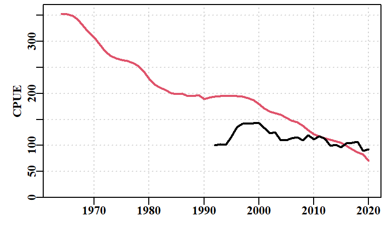
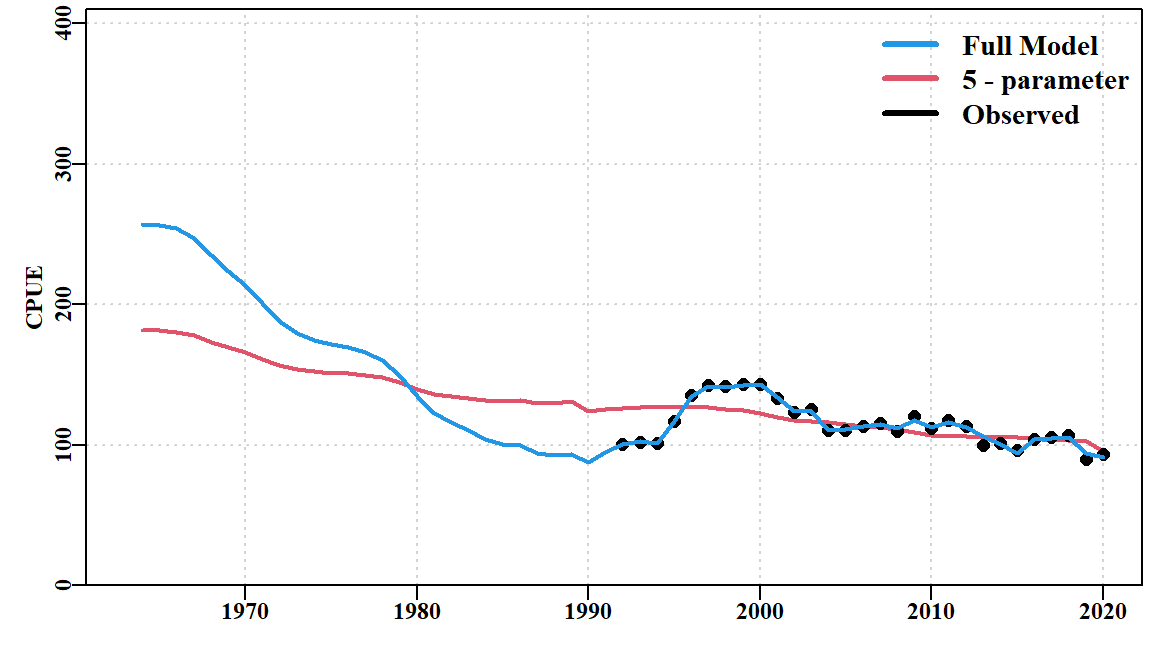
print(endtime - starttime)Time difference of 1.879251 secsWith only five parameters the model fit is generally very quick. Later, when we fit recruitment residuals the solution can take more time to be found. The improvement in model fit between the start and the 5-parameter fit is apparent both in the reduced total negative log-likelihood from 6462 to 2701, but in the reductions to both the log-likelihoods for CPUE (LLce) and the composition data (compL). When this model fit is plotted in full the improvement in fit to CPUE is also visible, although overall it remains poor, appearing to be a one-way decline.
Difference in equilibrium population Numbers-at-size > 10 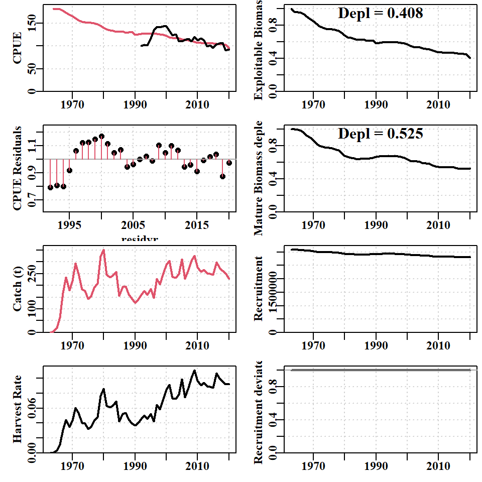
While the model fit will automatically provide an estimate of current depletion for both the mature biomass (important for recruitment dynamics) and exploitable biomass (important for the estimate of CPUE), it should be noted that the final predicted CPUE is well above the observed CPUE (Figure 6.5). The trends in the residuals also indicate that despite the improved model fit there remain some significant biases that demonstrate a serious model misspecification. The model has done its best to fit to the data, but the assumption of constant recruitment (bottom right panel) does not provide for sufficient flexibility for the modelled dynamics to be able to fit closely to the data.
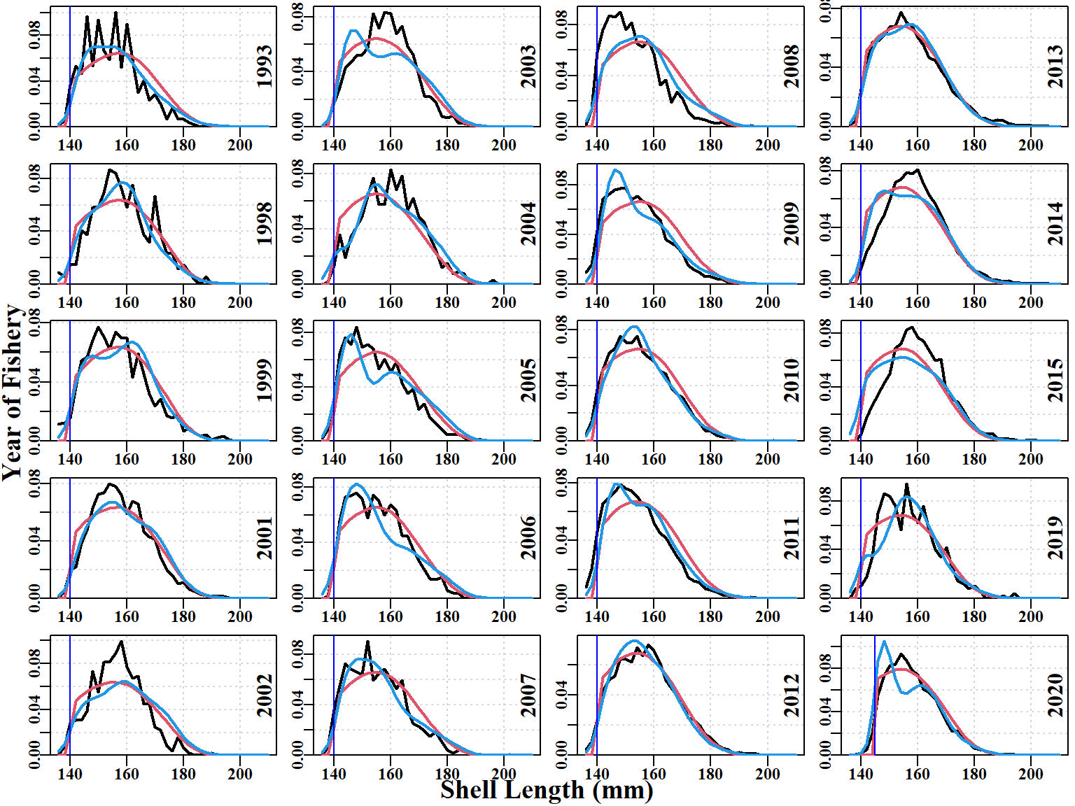
The fit to the size-composition data also has issues, although it is remarkably good in some years, in particular 2012, 2013, 2020 (Figure 6.6). Surprisingly, even the earlier years from 1994 to 2006, where sample sizes were relatively small, the fits that were produced are clearly approximating the distributions despite the noisiness of the data. Notice that some years, when the data were first considered (2014, 2015, and 2019), appear unusual in that the rising edge of the commercial data is right shifted away from the LML.
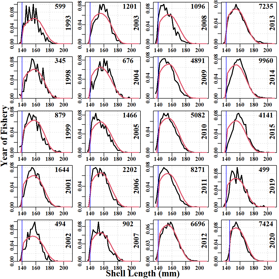
Importantly, the descending edge of the observed and fitted size-composition distribution, when compared to the theoretical unfished distribution contributes evidence towards estimating the depletion in each year (assuming selectivity is not dome-shaped; the model implemented logistic selectivity).
6.3 The 35-Parameter Model Including Recruitment Deviates
To allow the estimation of recruitment deviates it is only necessary to alter the ‘phase’ column in pindat from zero to 1. This could be done in sub-groups gradually, if problems arose during the fitting process. Alternatively, if the model has problems converging on a biologically plausible solutions then one can manually adjust some of the recruitment deviates time-lagged prior to increases in CPUE to improve the initial fit of predicted CPUE to that observed. This approach is sometimes needed to aid in obtaining a final plausible model fit. However, for data from statistical block 12, model fitting was able to proceed directly to estimating 35 parameters. With this many parameters, each iteration in the minimization takes longer, though now that Rcpp routines have been included to speed the calculations the whole process is much faster than the original R only code.
pindat[6:35,"phase"] <- 1
pindat[6:35,"param"] <- 0.1
pindat[1:5,"param"] <- c(14.25,3.29,5.2,-0.46,1.36)
Now, when the model is refit to the data it will alter all those zeros to adjust the recruitment in each of those years (1985 - 2014) and thereby improve the fit to the CPUE and size-composition data.
modin <- getpin(pindat)
pin <- modin$pin
notfix <- modin$notfix  # in this case all parameters are not fixed
allpin <- modin$allpin
allpin[notfix] <- pin
oldlogL <- negLLP(pars=pin,funk=dynamics,initpar=modin$allpin,
                  biol=biol,glb=glb,fish=fish,constants=constants,
                  notfixed=modin$notfix,omega=omega,finalcomp=sizecomp,
                  fiscomp=fiscomp,full=TRUE)
Difference in equilibrium population Numbers-at-size > 10 starttime <- Sys.time()
outmod2 <- fitlbm(pindat,negLLP,funk=dynamics,biol=biol,glb=glb,fish=fish,
constants=constants,omega=omega,sizecomp=sizecomp,
fiscomp=fiscomp,both=TRUE)initial value 2845.113909 iter 10 value 1407.251819
iter 20 value 1354.454309
iter 30 value 1333.216319
iter 40 value 1328.034588
iter 50 value 1327.222530
iter 60 value 1326.524064
iter 70 value 1325.738847
iter 80 value 1325.237478
iter 90 value 1324.613119
iter 100 value 1323.847725
iter 110 value 1323.340747
iter 120 value 1323.224617
iter 130 value 1323.127476
iter 140 value 1323.085858
iter 150 value 1323.082623
iter 150 value 1323.082623
iter 150 value 1323.082622
final value 1323.082622
converged
0: 1323.0826: 14.0987 3.33405 5.18416 -0.433344 1.40928 0.0578526 0.129311 0.227778 -0.254128 0.773467 0.805066 0.445180 0.200832 0.423153 0.533578 0.0481762 -0.140197 0.435316 -1.27799 0.513452 0.395607 0.363445 0.116582 0.819583 0.0648155 0.595222 0.117573 0.0616644 0.0915990 -0.267316 0.796522 0.328776 0.501531 -1.10073 0.890477
25: 1323.0799: 14.0982 3.33385 5.18448 -0.433050 1.41080 0.0593352 0.132020 0.233038 -0.250369 0.770941 0.808362 0.444856 0.202573 0.422683 0.533153 0.0479880 -0.140003 0.436237 -1.27846 0.515117 0.395481 0.363972 0.118817 0.820425 0.0653228 0.595210 0.116981 0.0615609 0.0929899 -0.265075 0.795719 0.332357 0.500808 -1.09839 0.890727
50: 1323.0613: 14.0769 3.33441 5.18561 -0.425872 1.41083 0.252045 0.267807 0.233927 -0.190501 0.793396 0.841358 0.445018 0.234640 0.426804 0.551504 0.0671789 -0.124130 0.455780 -1.28758 0.533297 0.410752 0.376703 0.139459 0.833419 0.0852341 0.608918 0.135467 0.0779464 0.107331 -0.236060 0.802577 0.364037 0.500774 -0.989233 0.894203
Difference in equilibrium population Numbers-at-size > 10 fitpar <- outmod2$ans2$par
optpar2 <- fitpar
neglogL <- negLLP(pars=fitpar,initpar=optpar2,funk=dynamics,biol=biol,
glb=glb,fish=fish,constants=constants,
notfixed=modin$notfix,omega=omega,finalcomp=sizecomp,
fiscomp=fiscomp,full=TRUE)Difference in equilibrium population Numbers-at-size > 10 likelihoods <- cbind(oldlogL,neglogL,(abs(oldlogL - neglogL)))
print(round(likelihoods[1:12,],4)) oldlogL neglogL
LLce 1427.5735 -68.0738 1495.6473
compL 1411.6218 1390.3194 21.3024
penaltyR 0.0000 0.0000 0.0000
sigmaCE 0.0337 0.0337 0.0000
wtsc 0.0070 0.0070 0.0000
penLnR0 0.2821 0.0937 0.1884
penDL 0.0000 0.0000 0.0000
pencatch 0.0000 0.0000 0.0000
penH 5.6366 0.7218 4.9148
penaltyCE 0.0000 0.0000 0.0000
totalL 2845.1139 1323.0610 1522.0529
sad 659.8509 34.2540 625.5969 pindat[modin$notfix,"param"] <- fitpar
endtime <- Sys.time()
print(endtime - starttime)Time difference of 49.7198 secsThe negative log-likelihoods have improved in that the LLce for CPUE has decreased from 67.606 in the 5-parameter fit to -68.074 and the compL for the size-composition data has decreased from 1458 down to 1390. When the data streams are completely consistent with each other and if the recruitment penalty has been omitted, the minimizer would have kept working until the fit to the CPUE and size-composition can be as perfect as possible. Not surprisingly, the resulting dynamics are rather different from that produced by the size-structured surplus-production model version. Other details of the model fit, such as the various penalties and limits are explained in the documentation to sizemod. sizemod includes a bias-ramp on the recruitment deviates, uses the Francis (2013) weighting on the cpue index of relative abundance, and iterative re-weighting of the relative weight given to the size-composition data. Once again, these details are described in detail and explained in sizemod’s documentation; using the built-in data sets these details have already been attended to in the example.
Difference in equilibrium population Numbers-at-size > 10 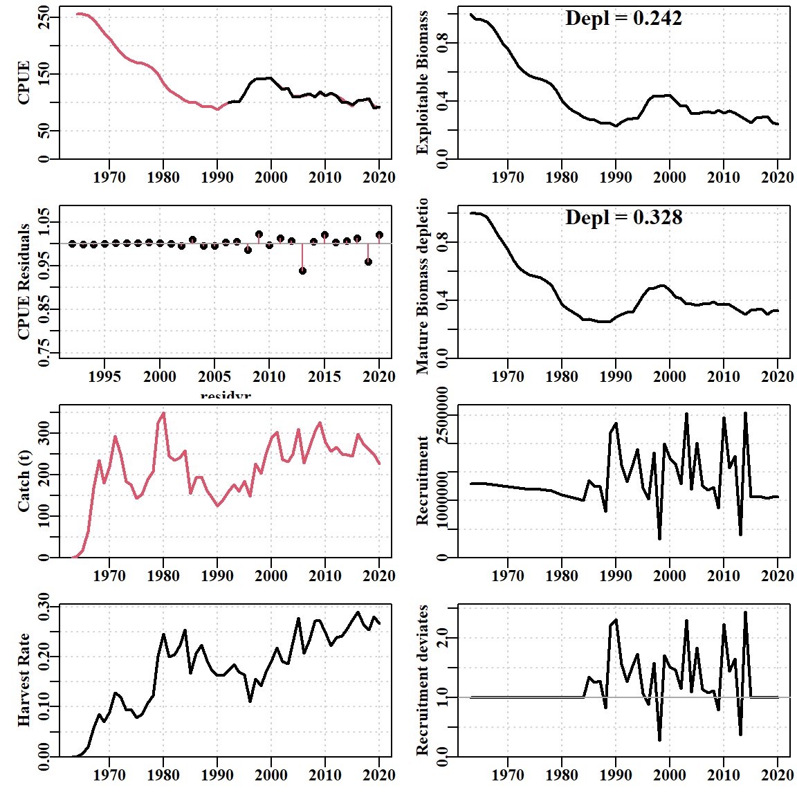
Comparing the model fits to the size-composition data (Figure 6.10) illustrates that the differences are more subtle than with the CPUE. Nevertheless, clear improvements are exhibited by the modified expected numbers-at-size in the catch. There are numerous improvements in the fits to the earlier noisy years of data, whereas in the years with larger samples the improvements are seemingly negligible or more subtle. However, for example, in the 2011 data the fit to the descending limb of the distribution is a clear improvement, as is the increased height of the rising limb.
6.3.1 Non-Linearity of CPUE
The situation modelled in this scenario used a \(\lambda = 0.75\). This may be understood by examining the following equation:
\[ \hat{I_t}=qB_t^{\lambda} \tag{6.1}\]
where \(\hat{I_t}\) is the predicted CPUE in year \(t\), \(q\) is the catchability, \(B_t\) is the exploitable biomass in year \(t\), and \(\lambda\) is a parameter that can alter the relationship between CPUE and exploitable biomass. In most stock assessments, \(\lambda = 1\) is assumed, which asserts a linear relationship. By using \(\lambda = 0.75\) the relationship between curvi-linear, which when illustrated clarifies the implications of the equation (Equation 6.1).
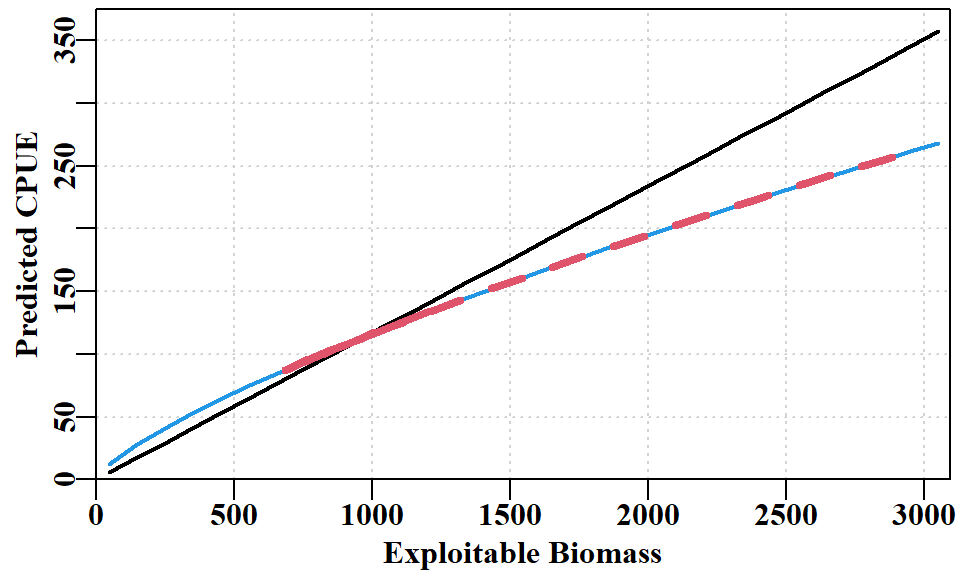
Note that the maximum CPUE predicted when \(\lambda = 0.75\) is 100kg/hr lower than if a linear relationship was used. This value appeared to divers to be more realistic when the fishery first started, as, at that time, handling time would have been much greater, and the risk of disturbing other abalone when removing one would mean many would lock down leading to damage if removal were attempted.
6.4 Initial Discussion
A classical, purely biomass based surplus production model can fit the abalone data remarkably well (Haddon, 2011, 2021), however, it only provides estimates of productivity and no information on the size-composition of the catch or the growth parameters. It also turns out to be relatively unstable for some of the statistical blocks and is extremely sensitive to variation in its parameters, especially the r parameter. The 5-parameter size-structured surplus production model has at least three advantages over the classical biomass-dynamic model:
by including the available size-composition data it can provide information concerning selectivity and growth as well as fishing mortality and final depletion (it can also inform about recruitment deviations but not in the 5-parameter model),
it can more easily model the dynamics that include the full history of catches, and
it is more stable when implementing non-linear relationships between the CPUE and exploitable biomass. Despite these advantages the observed fit to the CPUE data does not appear as good as that in the biomass-based surplus production model.
On the other hand, the 5-parameter model is also being fitted to the size-composition data so the model fit ends as a compromise between fitting the CPUE data and the size-composition data.
In its turn, the full 35-parameter model has an important advantage over the size-structured surplus-production model in that it can directly estimate the recruitment residuals required to adjust the model fits to both the CPUE (Figure 6.9) and the size-composition data (Figure 6.10).
Ignoring the recruitment deviates, the initial five parameter estimates also differ between the 5-parameter and the 35-parameter models:
| 5-param | 35-param | |
|---|---|---|
| LnR0 | 3081586 | 1327381 |
| MaxDL | 23.685 | 28.052 |
| L95 | 169.088 | 178.423 |
| qest | 0.2900 | 0.6483 |
| seldelta | 0.006 | 4.093 |
Much of the variation in CPUE is accounted for by the implementation of recruitment deviates in the 35-parameter model. Hence the differences between parameter values appear relatively large as they reflect differences in how productivity is expressed (more due to growth and less due to the average unfished recruitment in the 35-parameter model). Such changes were required to account for the changed dynamics when recruitment deviates were included. In fact, given these are numerical solutions, it is possible, if the initial parameter values are varied, to obtain essentially identical final model fits where the total likelihood differs at the second or third decimal place (of the order of a 10,000th of a percent difference). It is the case that, given the highly variable size-composition data and the highly variable catch data from year to year, a good deal of uncertainty can be expressed in the model outputs.
There are also some strong assumptions included in the assessment that are associated with the constant values given to some important parameters. These strong assumptions include that the natural mortality = 0.15, that the steepness of the Beverton-Holt stock recruitment relationship was 0.7, and that the lambda parameter, describing the non-linearity between CPUE and exploitable biomass, was 0.75. These values were fixed because for abalone they remain unknown or, at best, estimated for very small samples from few populations. Varying these parameters does not affect the model fit very much but does alter the implied unfished CPUE. In summary, the mathematical optimum model fit is different from the optimum biologically plausible model fit (initial catch rates staying within plausible values). The three assumed values appear to provide for the best compromise between optimizing both the statistical fit and the most biologically plausible set of implied population dynamics.
It has been demonstrated that it is possible, for a statistical block in Tasmania, to use the size-structured integrated assessment model to estimate the block’s productivity, the selectivity characteristics, the growth characteristics, and a series of recruitment deviates used to help describe the history of dynamics for which data are available. The uncertainty over what values to attribute to natural morality (\(M\)), recruitment steepness (\(h\)), and the non-linearity parameter (\(\lambda\)) remains a problem. Nevertheless, the use of the size-based integrated assessment to characterize the dynamics within each SAU is a great improvement over the simpler surplus production models.
6.5 Final Adjustments once in aMSE
After transferring the parameters from the sizemod estimates into each SAU within the aMSE operating model further adjustments are required to the AvRec and recruitment deviates to optimize the fits between the predicted CPUE at the SAU level and the observed standardized CPUE as well as optimizing the fits between the predicted size-composition of catch and those observed. This is done within aMSE using the two functions adjustavrec() and optimizerecdevs() (see their individual help pages within aMSE for their arguments and the syntax for how to use them.
The differences between the predicted MSY and AvRec for sizemod and aMSE is such that for each SAU in the Tasmanian western zone the MSY in aMSE is about 9.5% less than the sizemod estimate for each SAU, and the AvRec is about 3.8% larger in aMSE, although that relationship is much more variable between SAU. These differences between the sizemod and the aMSE values are a result of the dynamics in aMSE being split between each SAU’s populations rather than a single dynamic-pool within each SAU and the scale of the differences alters with the number of populations used within an SAU.