Chapter 7 Surplus Production Models
7.1 Introduction
In the previous chapters we have used and fitted what we have called static models that are stable through time (e.g. growth models using vB(), Gz(), or mm()). In addition, in the chapters Model Parameter Estimation and On Uncertainty, we have already introduced surplus production models (spm), that can be used to provide a stock assessment (e.g. the Schaefer model) and provide an example of dynamic models that use time-series of data. However, the development of the details of such models has been limited while we have focussed on particular modelling methods. Here we will examine surplus production models in more detail.
Surplus production models (alternatively Biomass Dynamic models; Hilborn and Walters, 1992) pool the overall effects of recruitment, growth, and mortality (all aspects of production) into a single production function dealing with undifferentiated biomass (or numbers). The term “undifferentiated” implies that all aspects of age and size composition, along with gender and other differences, are effectively ignored.
To conduct a formal stock assessment it is necessary, somehow, to model the dynamic behaviour and productivity of an exploited stock. A major component of these dynamics is the manner in which a stock responds to varied fishing pressure through time, that is, by how much does it increase or decrease in size. By studying the effects of different levels of fishing intensity it is often possible to assess a stock’s productivity. Surplus production models provide for the simplest stock assessments available that attempt to generate a description of such stock dynamics based on fitting the model to data from the fishery.
In the 1950s, Schaefer (1954, 1957) described how to use surplus production models to generate a fishery’s stock assessment. They have been developed in many ways since (Hilborn and Walters, 1992; Prager, 1994; Haddon, 2011; Winker et al, 2018) and it is a rapid survey of these more recent dynamic models that we will consider here.
7.1.1 Data Needs
The minimum data needed to estimate parameters for modern discrete versions of such models are at least one time-series of an index of relative abundance and an associated time-series of catch data. The catch data can cover more years than the index data. The index of relative stock abundance used in such simple models is often catch-per-unit-effort (cpue) but could be some fishery-independent abundance index (e.g., from trawl surveys, acoustic surveys), or both could be used.
7.1.2 The Need for Contrast
Despite occasional more recent use (Elder, 1979; Saila et al, 1979; Punt, 1994; Haddon, 1998), the use of surplus production models appears to have gone out of fashion in the 1980s. This was possibly because early on in their development it was necessary to assume the stocks being assessed were in equilibrium (Elder, 1979; Saila et al, 1979), and this often led to overly optimistic conclusions that were not supportable in the longer term. Hilborn (1979) analyzed many such situations and demonstrated that the data used were often too homogeneous; they lacked contrast in their effort levels and hence were uninformative about the dynamics of the populations concerned. For the data to lack contrast means that fishing catch and effort information is only available for a limited range of stock abundance levels and limited fishing intensity levels. A limited effort range means the range of responses to different fishing intensity levels will also be limited. A lack of such contrast can also arise when the stock dynamics are driven more by environmental factors than by the catches so that the stock can appear to respond to the fishery in unexpected ways (e.g. large changes to the stock despite no changes in catch or effort).
A strong assumption made with surplus production models is that the measure of relative abundance used provides an informative index of the relative stock abundance through time. Generally, the assumption is that there is a linear relationship between stock abundance and cpue, or other indices (though this is not necessarily a 1:1 relationship). The obvious risk is that this assumption is either false or can be modified depending on conditions. It is possible that cpue, for example, may become hyper-stable, which means it does not change even when a stock declines or increases. Or the variation of the index may increase so much as a result of external influences that detection of an abundance trend becomes impossible. For example, very large changes in cpue between years may be observed but not be biologically possible given the productivity of a stock (Haddon, 2018).
A different but related assumption is that the quality of the effort and subsequent catch-rates remains the same through time. Unfortunately, the notion of ‘effort creep’ as a result of technological changes in fishing gear, changes in fishing behaviour or methods, or other changes in fishing efficiency, is invariably a challenge or problem for assessments that rely on cpue as an index of relative abundance. The notion of effort-creep implies that the effectiveness of effort increases so that any observed nominal cpue, based on nominal effort, will over-estimate the relative stock abundance (it is biased high). Statistical standardization of cpue (Kimura, 1981; Haddon, 2018) can address some of these concerns but obviously can only account for factors for which data is available. For example, if one introduces GPS plotters or colour echo-sounders into a fishery, which would tend to increase the effectiveness of effort, but have no record of which vessels introduced them and when, their positive influence on catch rates would not be able to be accounted for by standardization.
7.1.3 When are Catch-Rates Informative
A possible test of whether the assumed relationship between abundance and any index of relative abundance is real and informative can be derived from the implication that, in a developed fishery, if catches are allowed to increase then it is expected that cpue will begin to decline some time after. Similarly, if catches are reduced to be less than surplus production, perhaps through management or marketing changes, then cpue would be expected to increase some time soon after as stock size increases. The idea being that if catches are less than the current productivity of a stock then eventually the stock size and thereby cpue should increase and vice-versa. If catches declined through a lack of availability but stayed at or above the current productivity then, of course, the cpue could not increase and may even decline further despite, perhaps minor, reductions in catch. Emphasis was placed upon developed fisheries because when a fishery begins, any initial depletion of the biomass will lead to “windfall” catches (MacCall, 2009) as the stock is fished down, which in turn will lead to cpue levels that would not be able to be maintained once a stock has been reduced away from unfished levels.
The expectation is, therefore, that in a developed fishery cpue would be, in many cases, negatively correlated with catches, possibly with a time-lag between cpue changing in response to changes in catches. If we can find such a relationship this usually means there is some degree of contrast in the data, if we cannot find such a negative relationship this generally means the information content of the data, with regard to how the stock responds to the fishery, is too low to inform an assessment based only on catches and the index of relative abundance. That is, the cpue adds little more information that that available in the catches.
We will use the MQMF data-set schaef to illustrate these ideas. schaef contains the catches and cpue of the original yellow-fin tuna data from Schaefer (1957), which was an early example of the use of surplus production models to conduct stock assessments.
| year | catch | effort | cpue | year | catch | effort | cpue |
|---|---|---|---|---|---|---|---|
| 1934 | 60913 | 5879 | 10.3611 | 1945 | 89194 | 9377 | 9.5120 |
| 1935 | 72294 | 6295 | 11.4844 | 1946 | 129701 | 13958 | 9.2922 |
| 1936 | 78353 | 6771 | 11.5719 | 1947 | 160134 | 20381 | 7.8570 |
| 1937 | 91522 | 8233 | 11.1165 | 1948 | 200340 | 23984 | 8.3531 |
| 1938 | 78288 | 6830 | 11.4624 | 1949 | 192458 | 23013 | 8.3630 |
| 1939 | 110417 | 10488 | 10.5279 | 1950 | 224810 | 31856 | 7.0571 |
| 1940 | 114590 | 10801 | 10.6092 | 1951 | 183685 | 18726 | 9.8091 |
| 1941 | 76841 | 9584 | 8.0176 | 1952 | 192234 | 31529 | 6.0971 |
| 1942 | 41965 | 5961 | 7.0399 | 1953 | 138918 | 36423 | 3.8140 |
| 1943 | 50058 | 5930 | 8.4415 | 1954 | 138623 | 24995 | 5.5460 |
| 1944 | 64094 | 6397 | 10.0194 | 1955 | 140581 | 17806 | 7.8951 |
The plot of catch, cpue, and their relationship, Figure(7.1), only exhibits a weak negative relationship between cpue and catch. If we examine the outcome of the regression conducted using lm() by using summary(model), we find this regression is only just significant at P = 0.04575. However, this reflects a correlation with no time-lags, i.e. a lag = 0. We do not know how many years may need to pass before we can detect a potential effect of a change in catch on cpue, so hence, we need to do a time-lagged correlation analysis between cpue and catch; for that we can use the base R cross-correlation function ccf().
 #schaef fishery data and regress cpue and catch    Fig 7.1
parset(plots=c(3,1),margin=c(0.35,0.4,0.05,0.05))
plot1(schaef[,"year"],schaef[,"catch"],ylab="Catch",xlab="Year",
      defpar=FALSE,lwd=2)
plot1(schaef[,"year"],schaef[,"cpue"],ylab="CPUE",xlab="Year",
      defpar=FALSE,lwd=2)
plot1(schaef[,"catch"],schaef[,"cpue"],type="p",ylab="CPUE",
      xlab="Catch",defpar=FALSE,pch=16,cex=1.0)
model <- lm(schaef[,"cpue"] ~ schaef[,"catch"])
abline(model,lwd=2,col=2) # summary(model) 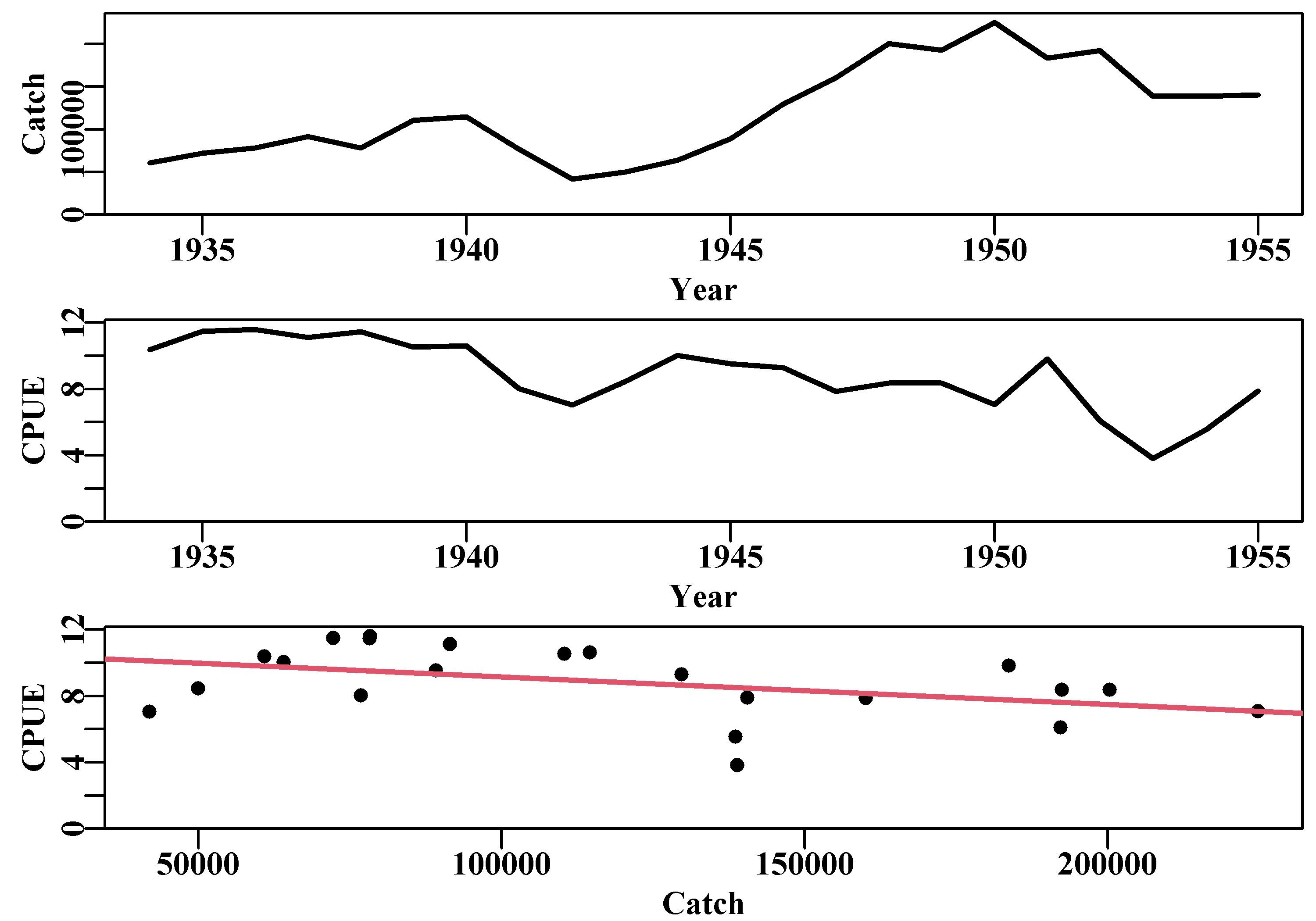
Figure 7.1: The catches and cpue by year, and their relationship, described by a regression, for the Schaefer (1957) yellowfin tuna fishery data.
As before there is an indication that a time-lag = 0 is only just significant. However, the significant negative correlation of cpue on catch at a lag of 2 years, Figure(7.2), suggests that there would be sufficient contrast in this yellow-fin tuna data to inform a surplus production model (there are also significant effects at 1, 3, and 4 years). This correlation should become more apparent if we physically lag the CPUE data by two year, Figure(7.3).
 #cross correlation between cpue and catch in schaef Fig 7.2
parset(cex=0.85) #sets par parameters for a tidy base graphic
ccf(x=schaef[,"catch"],y=schaef[,"cpue"],type="correlation",
ylab="Correlation",plot=TRUE) 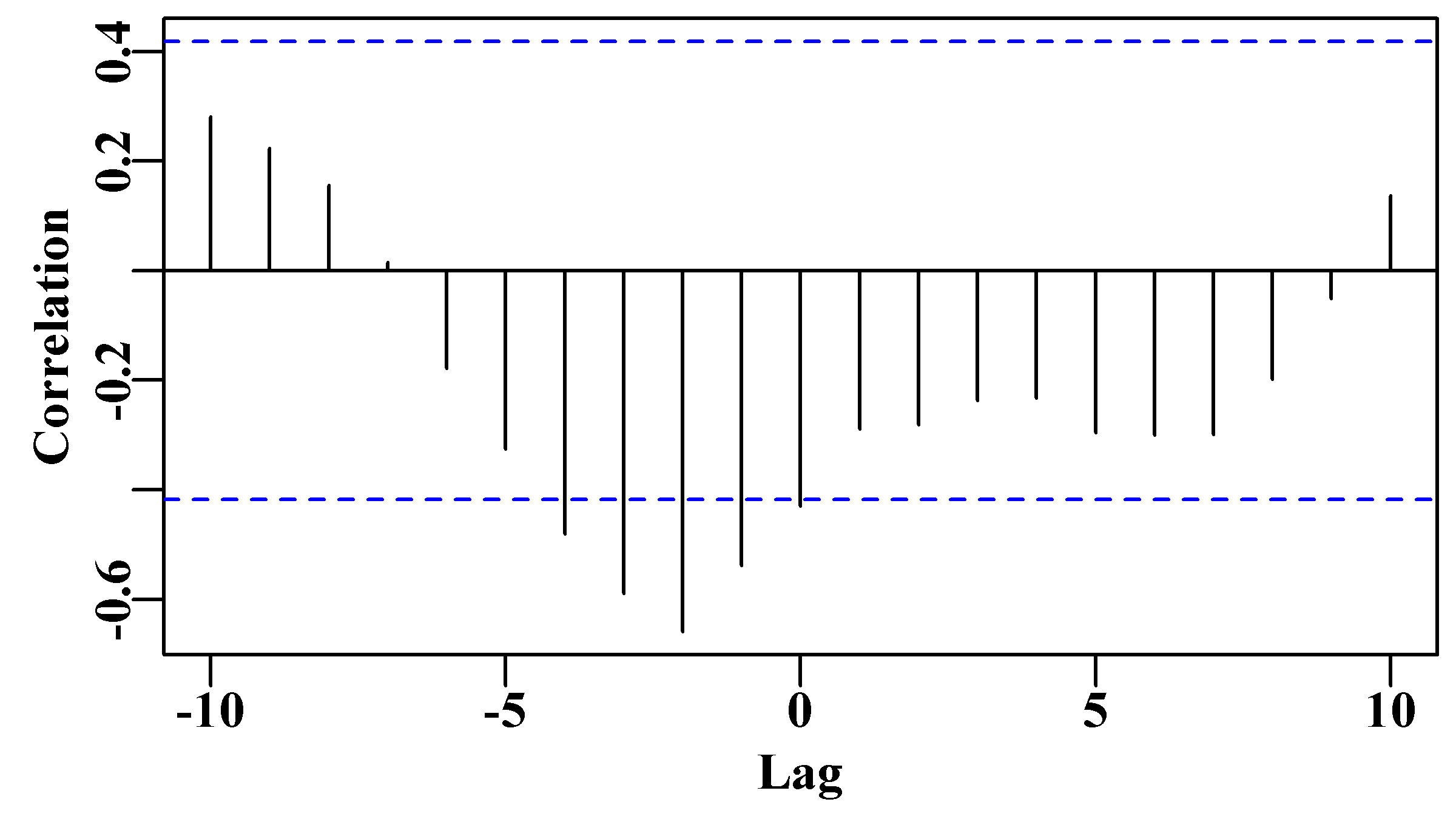
Figure 7.2: The cross correlation between catches and cpue for the Schaefer (1957) yellowfin tuna fishery data (schaef) obtained using the ccf() function in R. The blue dashed lines denote the significant correlation levels.
 #now plot schaef data with timelag of 2 years on cpue   Fig 7.3
parset(plots=c(3,1),margin=c(0.35,0.4,0.05,0.05))
plot1(schaef[1:20,"year"],schaef[1:20,"catch"],ylab="Catch",
      xlab="Year",defpar=FALSE,lwd=2)
plot1(schaef[3:22,"year"],schaef[3:22,"cpue"],ylab="CPUE",
      xlab="Year",defpar=FALSE,lwd=2)
plot1(schaef[1:20,"catch"],schaef[3:22,"cpue"],type="p",
      ylab="CPUE",xlab="Catch",defpar=FALSE,cex=1.0,pch=16)
model2 <- lm(schaef[3:22,"cpue"] ~ schaef[1:20,"catch"])
abline(model2,lwd=2,col=2) 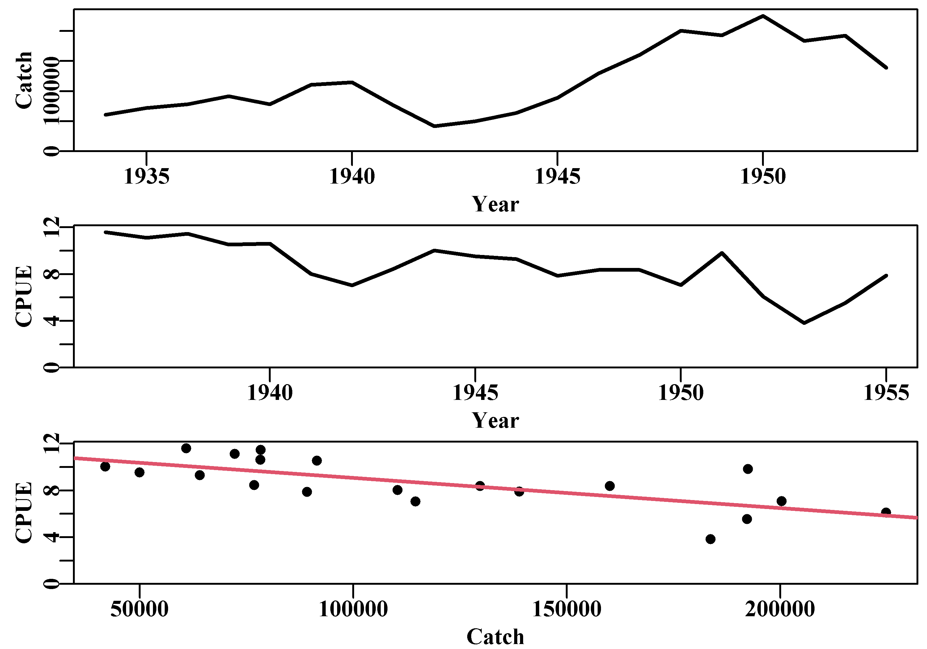
Figure 7.3: The catches and cpue, and their relationship, for the Schaefer (1957) yellowfin tuna fishery data. With a negative lag of 2 years on the cpue time-series the negative or inverse correlation becomes more apparent.
The relationship between cpue and catches from the Schaefer (1957) yellowfin tuna fishery data with a negative lag of 2 years imposed on the cpue time-series (rows 3:22 against row 1:20). The very small gradient is a reflection of the catches being reported in ’000s of pounds.
#
# Call:
# lm(formula = schaef[3:22, "cpue"] ~ schaef[1:20, "catch"])
#
# Residuals:
#      Min       1Q   Median       3Q      Max
# -3.10208 -0.92239 -0.06399  1.04280  3.11900
#
# Coefficients:
#                         Estimate Std. Error t value Pr(>|t|)
# (Intercept)            1.165e+01  7.863e-01  14.814 1.59e-11
# schaef[1:20, "catch"] -2.576e-05  6.055e-06  -4.255 0.000477
#
# Residual standard error: 1.495 on 18 degrees of freedom
# Multiple R-squared:  0.5014,  Adjusted R-squared:  0.4737
# F-statistic:  18.1 on 1 and 18 DF,  p-value: 0.0004765
7.2 Some Equations
The dynamics of the stock being assessed are described using an index of relative abundance. The index, however it is made, is assumed to reflect the biomass available to the method used to estimate it (fishery-dependent cpue or an independent survey) and this biomass is assumed to be affected by the catches removed by the fishery. This means, if we are using commercial catch-per-unit-effort (cpue), that strictly we are dealing with the exploitable biomass and not the spawning biomass (which is the more usual objective of stock assessments). However, generally, the assumption is made that the selectivity of the fishery is close to the maturity ogive so that the index used is still indexing spawning biomass, at least approximately. Even so, exactly what is being indexed should be considered explicitly before drawing such conclusions.
In general terms, the dynamics are designated as a function of the biomass at the start of a given year t, though it could, by definition, refer to a different date within a year. Remember that the end of a year is effectively the same as the start of the next year although precisely which is used will influence how to start and end the analysis (e.g. from which biomass-year to remove the catches taken in a given year):
\[\begin{equation} \begin{split} {B_0} &= {B_{init}} \\ {B_{t+1}} &= {B_t}+r{B_t}\left( 1-\frac{{B_t}}{K} \right)-{C_t} \end{split} \tag{7.1} \end{equation}\]
where \(B_{init}\) is the initial biomass at whatever time one’s data begins. If data is available from the beginning of fishery then \(B_{init} = K\), where \(K\) is the carrying capacity or unfished biomass. \(B_t\) represents the stock biomass at the start of year \(t\), \(r\) represents the population’s intrinsic growth rate, and \(r{B_t}\left( 1-\frac{{B_t}}{K} \right)\) represents a production function in terms of stock biomass that accounts for recruitment of new individuals, any growth in the biomass of current individuals, natural mortality and assumes linear density-dependent effects on population growth rate. Finally, \(C_t\) is the catch during the year \(t\), which represents fishing mortality. The emphasis placed upon when in the year each term refers to is important, as it determines how the dynamics are modelled in the equations and the consequent R code.
In order to compare and then fit the dynamics of such an assessment model with the real world the model dynamics are also used to generate predicted values for the index of relative abundance in each year:
\[\begin{equation} \hat {I}_{t}=\frac{{C}_{t}}{{E}_{t}}=q{B}_{t} \tag{7.2} \end{equation}\]
where \(\hat {I}_{t}\) is the predicted or estimated mean value of the index of relative abundance in year \(t\), which is compared to the observed indices to fit the model to the data, \(E_t\) is the fishing effort in year \(t\), and \(q\) is the catchability coefficient (defined as the amount of biomass/catch taken with one unit of effort). This relationship also makes the strong assumption that the stock biomass is what is known as a dynamic-pool. This means that irrespective of geographical distance, any influences of the fishery, or the environment, upon the stock dynamics have an effect across the whole stock within each time-step used (often one year but could be less). This is a strong assumption, especially if any consistent spatial structure occurs within a stock or the geographical scale of the fishery is such that large amounts of time would be needed for fish in one region to travel to a different region. Again, awareness of these assumptions is required to appreciate the limitations and appropriately interpret any such analyses.
7.2.1 Production Functions
A number of functional forms have been put forward to describe the productivity of a stock and how it responds to stock size. We will consider two, the Schaefer model and a modified form of the Fox (1970) model, plus a generalization that encompasses both:
The production function of the Schaefer (1954, 1957) model is:
\[\begin{equation} f\left( {B}_{t}\right)=r{B}_{t}\left( 1-\frac{{B}_{t}}{K} \right) \tag{7.3} \end{equation}\]
while a modified version of the Fox (1970) model uses:
\[\begin{equation} f\left( {B_t}\right)=\log({K})r{B}_{t}\left( 1-\frac{\log({B_t})}{\log({K})}\right) \tag{7.4} \end{equation}\]
The modification entails the inclusion of the \(\log(K)\) as the first term, which only acts to maintain the maximum productivity at approximately the equivalent of a similar set of parameters in the Schaefer model.
Pella and Tomlinson (1969) produced a generalized production function that included the equivalent to both the Schaefer and the Fox model as special cases. Here, we will use an alternative to their formulation that was produced by Polacheck et al (1993). This provides a general equation for the population dynamics that can be used for both the Schaefer and the Fox model, and gradations between, depending on the value of a single parameter p.
\[\begin{equation} {B}_{t+1}={B}_{t}+{rB_t}\frac{1}{p}\left( 1- \left(\frac{{B}_{t}}{K} \right)^p \right)-{{C}_{t}} \tag{7.5} \end{equation}\]
where the first term, \(B_t\), is the stock biomass at time \(t\), and the last term is
\(C_t\), which is the catch taken in time \(t\). The middle term is a more complex component that defines the production curve. This is made up of \(r\), the intrinsic rate of population growth, \(B_t\), the current biomass at time \(t\), \(K\), the carrying capacity or maximum population size, and \(p\) is a term that controls any asymmetry of the production curve. If \(p\) is set to 1.0 (the default in the MQMF discretelogistic() function), this equation simplifies to the classical Schaefer model (Schaefer, 1954, 1957). Polacheck et al (1993) introduced the equation above, but it tends to be called the Pella-Tomlinson (1969) surplus production model (though their formulation was different it has very similar properties).
The sub-term \(rB_{t}\) represents unconstrained exponential population growth (because in this difference equation, it is added to \(B_t\)), which, as long as \(r > 0.0\), would lead to unending positive population growth in the absence of catches (such positive exponential growth is still exemplified by the world’s human population; although plague in the 14th century reversed that trend for a brief but particularly unhappy time). The sub-term \((1/p)(1 – (Bt/K)^p)\) provides a constraint on the exponential growth term because its value tends to zero as the population size increases. This acts as, and is known as, a density-dependent effect.
When p is set to 1.0 this equation becomes the same as the Schaefer model (linear density-dependence). But when p is set to a very small number, say 1e-08, then the formulation becomes equivalent to the Fox model’s dynamics. Values of p > 1.0 lead to a production curve skewed to the left with the mode to the right of center. With p either > 1 or < 1, the density-dependence would no longer be linear in character. Generally, one would fix the p value and not attempt to fit it using data. Catch and an index of relative abundance alone would generally be insufficient to estimate the detailed effect on productivity of relative population size.
 #plot productivity and density-dependence functions Fig7.4
prodfun <- function(r,Bt,K,p) return((r*Bt/p)*(1-(Bt/K)^p))
densdep <- function(Bt,K,p) return((1/p)*(1-(Bt/K)^p))
r <- 0.75; K <- 1000.0; Bt <- 1:1000
sp <- prodfun(r,Bt,K,1.0)  # Schaefer equivalent
sp0 <- prodfun(r,Bt,K,p=1e-08)  # Fox equivalent
sp3 <- prodfun(r,Bt,K,3) #left skewed production, marine mammal?
parset(plots=c(2,1),margin=c(0.35,0.4,0.1,0.05))
plot1(Bt,sp,type="l",lwd=2,xlab="Stock Size",
      ylab="Surplus Production",maxy=200,defpar=FALSE)
lines(Bt,sp0 * (max(sp)/max(sp0)),lwd=2,col=2,lty=2) # rescale
lines(Bt,sp3*(max(sp)/max(sp3)),lwd=3,col=3,lty=3)   # production
legend(275,100,cex=1.1,lty=1:3,c("p = 1.0 Schaefer","p = 1e-08 Fox",
                 "p = 3 LeftSkewed"),col=c(1,2,3),lwd=3,bty="n")
plot1(Bt,densdep(Bt,K,p=1),xlab="Stock Size",defpar=FALSE,
      ylab="Density-Dependence",maxy=2.5,lwd=2)
lines(Bt,densdep(Bt,K,1e-08),lwd=2,col=2,lty=2)
lines(Bt,densdep(Bt,K,3),lwd=3,col=3,lty=3) 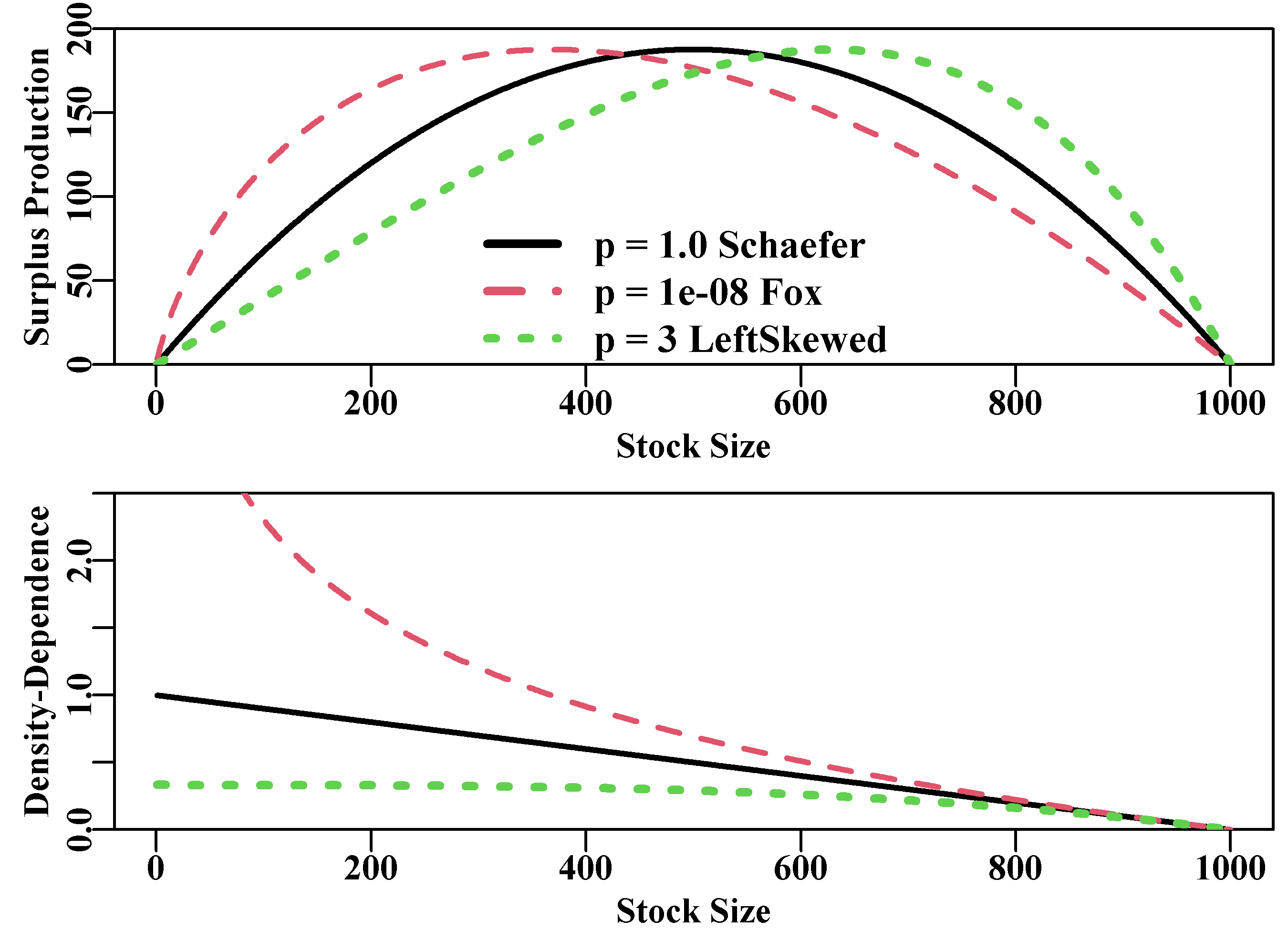
Figure 7.4: The effect of the p parameter on the Polacheck et al, 1993, production function (upper plot) and on the density-dependent term (lower plot). Note the rescaling of the productivity to match that produced by the Schaefer curve. Stock size could be biomass or numbers.
The Schaefer model assumes a symmetrical production curve with maximum surplus production or maximum sustainable yield (MSY) at \(0.5K\) and the density-dependent term trends linearly from 1.0 at very low population sizes to zero as \(B_t\) tends towards \(K\). The Fox model is approximated when p has a small value, say \(p=1e-08\), which generates an asymmetrical production curve with the maximum production at some lower level of depletion (in this case at \(0.368K\), found using Bt[which.max(sp0)]). The density-dependent term is non-linear and the maximum productivity (\(MSY\)) occurs where the density-dependent term = 1.0. Without the re-scaling used in Figure(7.4) the Fox model is generally more productive than the Schaefer as a result of the density-dependent term becoming greater than 1.0 at stock sizes less than \(B_{MSY}\), the stock biomass that generates \(MSY\). With values of p > 1.0, the maximum productivity occurs at higher stock sizes and with population growth rates increasing only almost linearly at lower stock sizes and density-dependent declines only occurring at rather higher stock levels. Such dynamics would be more typical of marine mammals than of fish.
The Schaefer model can be regarded as more conservative than the Fox in that it requires the stock size to be higher for maximum production and generally leads to somewhat lower levels of catch, though exceptions could occur because of the generally higher productivity from Fox-type models.
7.2.2 The Schaefer Model
For the Schaefer model we would set \(p = 1.0\) leading to:
\[\begin{equation} {B}_{t+1}={B}_{t}+r{B}_{t}\left( 1-\frac{{B}_{t}}{K} \right)-{C}_{t} \tag{7.6} \end{equation}\]
Given a time-series of fisheries data there will always be an initial biomass which might be \(B_{init} = K\), or \(B_{init}\) being some fraction of \(K\), depending on whether the stock was deemed to be depleted when data from the fishery first became available. It is also not impossible that \(B_{init}\) can be larger than \(K\), as real populations tend not to exhibit a stable equilibrium.
Fitting the model to data would require at least three parameters, the \(r\), the \(K\), and the catchability coefficient \(q\) (\(B_{init}\) might also be needed). However, it is possible to use what is known as a “closed-form” method for estimating the catchability coefficient \(q\):
\[\begin{equation} \hat{q}=\exp \left( \frac{1}{n}\sum{\log{\left( \frac{{I}_{t}}{\hat{B}_{t}} \right)}} \right) \tag{7.7} \end{equation}\]
which is the back-transformed geometric mean of the observed CPUE divided by the predicted exploitable biomass (Polacheck et al, 1993). This generates an average catchability for the time-series. In circumstances where a fishery has undergone a major change such that the quality of the CPUE has changed, it is possible to have different estimates of catchability for different parts of the time-series. However, care is needed to have a strong defense for such suggested model specifications, especially as the shorter the time-series used to estimate \(q\) the more uncertainty will be associated with it.
7.2.3 Sum of Squared Residuals
Such a model can be fitted using least squares or, more properly, the sum of squared residual errors:
\[\begin{equation} ssq=\sum{\left( \log({I}_{t}) - \log(\hat{I}_{t}) \right)}^{2} \tag{7.8} \end{equation}\]
the log-transformations are required as generally CPUE tends to be distributed log-normally and the least-squares method implies normal random errors. The least squares approach tends to be relatively robust when first searching for a set of parameters that enable a model to fit to available data. However, once close to a solution more modelling options become available if one then uses maximum likelihood methods. The full log-normal log likelihood is:
\[\begin{equation} L\left( data|{B}_{init},r,K,q \right)=\prod\limits_{t}{\frac{1}{{I}_{t}\sqrt{2\pi \hat{\sigma }}}{{e}^{\frac{-\left( \log{{I}_{t}}-\log{{\hat{I_t}}} \right)}{2{{{\hat{\sigma }}}^{2}}}}}} \tag{7.9} \end{equation}\]
Apart from the log transformations this differs from Normal PDF likelihoods by the variable concerned (here \(I_t\)) being inserted before the \(\sqrt{2\pi \hat{\sigma }}\) term. Fortunately, as shown in Model Parameter Estimation, the negative log-likelihood can be simplified (Haddon, 2011), to become:
\[\begin{equation} -veLL=\frac{n}{2}\left( \log(2\pi)+2\log(\hat\sigma)+ 1 \right) \tag{7.10} \end{equation}\]
where the maximum likelihood estimate of the standard deviation, \(\hat\sigma\) is given by:
\[\begin{equation} \hat{\sigma }=\sqrt{\frac{\sum{{{\left( \log({{I}_{t}})-\log( {{\hat{I_t}}}) \right)}^{2}}}}{n}} \tag{7.11} \end{equation}\]
Note the division by n rather than by n-1. Strictly, for the log-normal (in Equ(7.10)), the -veLL should be followed by an additional term:
\[\begin{equation} -\sum{\log({I_t})} \tag{7.12} \end{equation}\]
the sum of the log-transformed observed catch rates. But as this will be constant it is usually omitted. Of course, when using R we can always use the built in probability density function implementations (see negLL() and negLL1()) so such simplifications are not strictly necessary, but they can remain useful when one wishes to speed up the analyses using Rcpp, although Rcpp-syntactic-sugar, which leads to C++ code looking remarkably like R code, now includes versions of dnorm() and related distribution functions.
7.2.4 Estimating Management Statistics
The Maximum Sustainable Yield can be calculated for the Schaefer model simply by using:
\[\begin{equation} MSY=\frac{rK}{4} \tag{7.13} \end{equation}\]
However, for the more general equation using the p parameter from Polacheck et al (1993) one needs to use:
\[\begin{equation} MSY=\frac{rK}{\left(p+1 \right)^\frac{\left(p+1 \right)}{p}} \tag{7.14} \end{equation}\]
which simplifies to Equ(7.13) when \(p = 1.0\). We can use the MQMF function getMSY() to calculate Equ(7.14), which is one illustration of how the Fox model can imply greater productivity than the Schaefer.
 #compare Schaefer and Fox MSY estimates for same parameters
param <- c(r=1.1,K=1000.0,Binit=800.0,sigma=0.075)
cat("MSY Schaefer = ",getMSY(param,p=1.0),"\n") # p=1 is default
cat("MSY Fox      = ",getMSY(param,p=1e-08),"\n")
# MSY Schaefer = 275
# MSY Fox = 404.6674Of course, if you fit the two models to real data this will generally produce different parameters for each and so the derived MSY’s may be closer in value.
It is also possible to produce effort-based management statistics. The effort level that if maintained should lead the stock to achieve MSY at equilibrium is known as \(E_{MSY}\):
\[\begin{equation} E_{MSY} = \frac{r}{q(1+p)} \tag{7.15} \end{equation}\]
which collapses to \(E_{MSY} = r/2q\) for the Schaefer model but remains general for other values of the p parameter. It is also possible to estimate the equilibrium harvest rate (proportion of stock taken each year) that should lead to \(B_{MSY}\), which is the biomass that has a surplus production of MSY:
\[\begin{equation} H_{MSY} = qE_{MSY} = q \frac{r}{q+qp} = \frac{r}{1+p} \tag{7.16} \end{equation}\]
It is not uncommon to see Equ(7.16) depicted as \(F_{MSY} = qE_{MSY}\), but this can be misleading as \(F_{MSY}\) would often be interpreted as an instantaneous fishing mortality rate, whereas, in this case, it is actually a proportional harvest rate. For this reason I have explicitly used \(H_{MSY}\).
7.2.5 The Trouble with Equilibria
The real-world interpretation of management targets is not always straightforward. An equilibrium is now assumed to be unlikely in most fished populations, so the interpretation of MSY is more like an average, long-term expected potential yield if the stock is fished optimally; a dynamic equilibrium might be a better description. The \(E_{MSY}\) is the effort that, if consistently applied, should give rise to the MSY, but only if the stock biomass is at \(B_{MSY}\), the biomass needed to generate the maximum surplus production. Each of these management statistics is derived from equilibrium ideas. Clearly, a fishery could be managed by limiting effort to \(E_{MSY}\), but if the stock biomass starts of badly depleted, then the average long-term yield will not result. In fact, the \(E_{MSY}\) effort level may be too high to permit stock rebuilding in this non-equilibrium world. Similarly, \(H_{MSY}\), would operate as expected but only when the stock biomass was at \(B_{MSY}\). It would be possible to estimate the catch or effort level that should lead the stock to recover to \(B_{MSY}\), and this could be termed \(F_{MSY}\), but this would require conducting stock projections and searching for the catch levels that would eventually lead to the desired result. We will examine making population projections in later sections.
It is important to emphasize that the idea of \(MSY\) and its related statistics are based around the idea of equilibrium, which is a rarity in the real world. At best, a dynamic equilibrium may be achievable but, whatever the case, there are risks associated with the use of such equilibrium statistics. When it was first developed the concept of \(MSY\) was deemed a suitable target towards which to manage a fishery. Now, despite being incorporated into a number of national fisheries acts and laws as the overall objective of fisheries management, it is safer to treat \(MSY\) as an upper limit on fishing mortality (catch); a limit reference point rather than a target reference point.
Ideally, the outcomes from an assessment need to be passed through a harvest control rule (HCR) that provides for formal management advice, with regard to future catches or effort, in response to the estimated stock status (fishing mortality and stock depletion levels). However, few of these potential management outputs are of value without some idea of the uncertainty around their values. As we have indicated, it would also be very useful to be able to project the models into the future to provide a risk assessment of alternative management strategies. But first we need to fit the models to data.
7.3 Model Fitting
Details of the model parameters and other aspects relating to the model can also be found in the help files for each of the functions (try ?spm or ?simpspm). In brief, the model parameters are \(r\) the net population rate of increase (combined individual growth in weight, recruitment, and natural mortality), \(K\) the population carrying capacity or unfished biomass, and \(B_{init}\) is the biomass in the first year. This parameter is only required if the index of relative abundance data (usually cpue ) only becomes available after the fishery has been running for a few years implying that the stock has been depleted to some extent. If no initial depletion is assumed then \(B_{init}\) is not needed in the parameter list and is set equal to \(K\) inside the function. The final parameter is sigma, the standard deviation of the Log-Normal distribution used to describe the residuals. simpspm() and spm() are designed for use with maximum likelihood methods so even if you use ssq() as the criterion of optimum fit, a sigma value is necessary in the parameter vector.
In Australia the index of relative stock abundance is most often catch-per-unit-effort (cpue ), but could be some fishery-independent abundance index (e.g., from trawl surveys, acoustic surveys), or both could be used in one analysis (see simpspmM()). The analysis will permit the production of on-going management advice as well as a determination of stock status.
In this section we will describe the details of how to conduct a surplus production analysis, how to extract the results from that analysis as well as plot out illustrations of those results.
7.3.1 A Possible Workflow for Stock Assessment
When conducting a stock assessment based upon a surplus production model one possible work flow might include:
- read in time-series of catch and relative abundance data. It can help to have functions that check for data completeness, missing values, and other potential issues, but it is even better to know your own data and its limitations.
- use a
ccf()analysis to determine whether the cpue data relative to the catch data may be informative. If a significant negative relation was found this would strengthen any defense of the analysis.
- define/guess a set of initial parameters containing r and K, and optionally \(B_{init}\) = initial biomass, which is used if it is suspected that the fishery data starts after the stock has been somewhat depleted.
- use the function
plotspmmod()to plot up the implications of the assumed initial parameter set for the dynamics. This is useful when searching for plausible initial parameters sets.
- use
nlm()orfitSPM()to search for the optimum parameters once a potentially viable initial parameter set are input. See discussion.
- use
plotspmmod()using the optimum parameters to illustrate the implications of the optimum model and it relative fit (especially using the residual plot).
- ideally one should examine the robustness of the model fit by using multiple different initial parameter sets as starting points for the model fitting procedure, see
robustSPM(). - once satisfied with the robustness of the model fit, use
spmphaseplot()to plot out the phase diagram of biomass against harvest rate so as to determine and illustrate the stock status visually.
- use
spmboot(), asymptotic standard errors, or Bayesian methods from On Uncertainty, to characterize uncertainty in the model fit and outputs. Tabulating and plotting such outputs. See later.
- Document and defend any conclusions reached.
Two common versions of the dynamics are currently available inside MQMF: the classical Schaefer model (Schaefer, 1954) and an approximation to the Fox model (Fox, 1970; Polacheck et al, 1993), both are described in Haddon (2011). Prager (1994) provides many additional forms of analysis that are possible using surplus production models and practical implementations are also provided in Haddon (2011).
 #Initial model 'fit' to the initial parameter guess  Fig 7.5
data(schaef); schaef <- as.matrix(schaef)
param <- log(c(r=0.1,K=2250000,Binit=2250000,sigma=0.5))
negatL <- negLL(param,simpspm,schaef,logobs=log(schaef[,"cpue"]))
ans <- plotspmmod(inp=param,indat=schaef,schaefer=TRUE,
addrmse=TRUE,plotprod=FALSE) 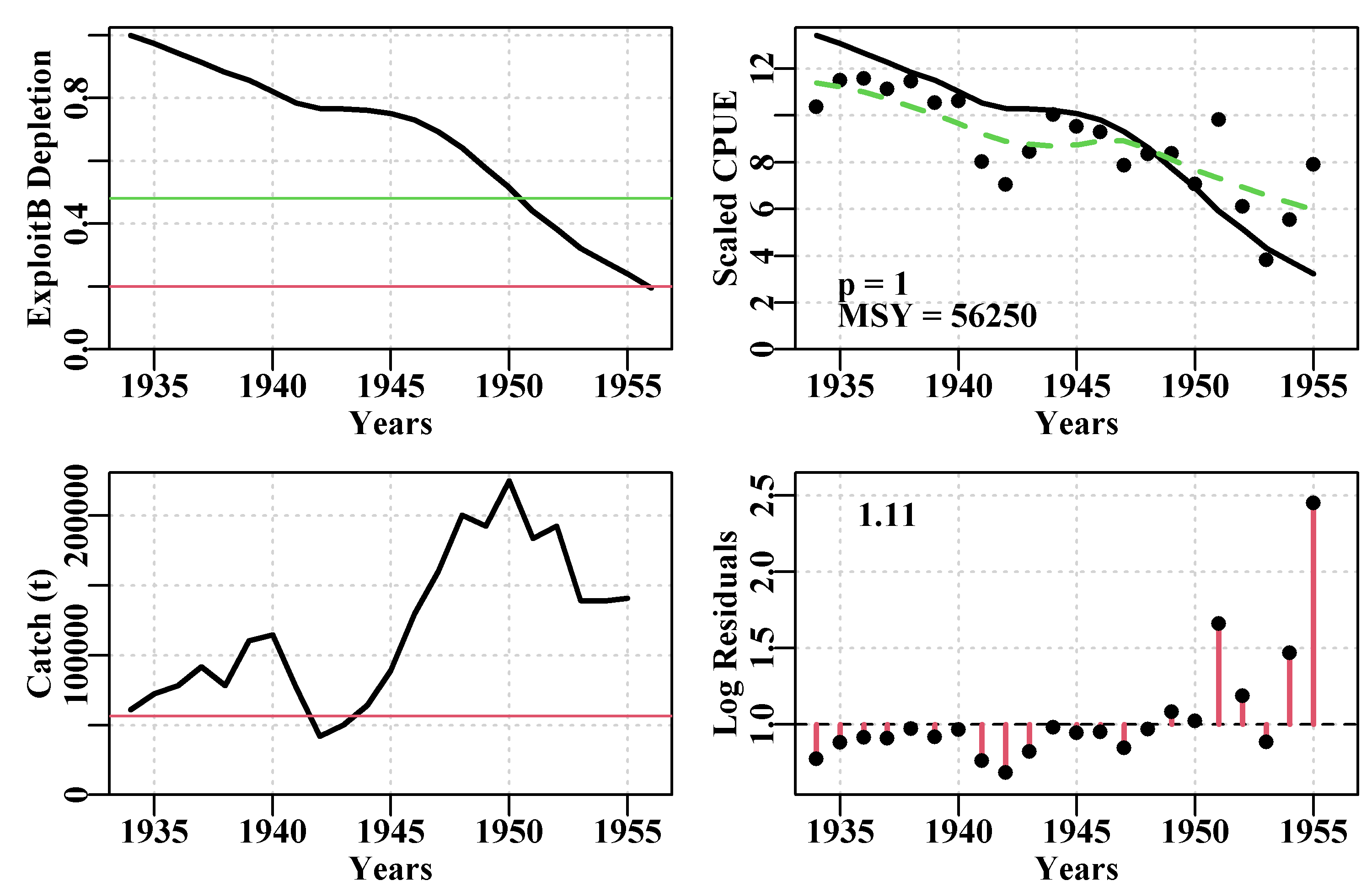
Figure 7.5: The tentative fit of a surplus production model to the schaef data-set using the initial parameter values. The dashed green line in the CPUE plot is a simple loess fit, while the solid line is that implied by the guessed input parameters. The horizontal red line in the catch plot is the predicted MSY. The number in the residual plot is the root mean square error of the log-normal residuals.
The r value of 0.1 leads to a negatL = 8.2877, and a strong residual pattern of all residuals below 1.0 up to about 1950 and four large and positive residuals afterwards. The K value was set at about 10 times the maximum catch and something of that order (10x to 20x) will often lead to sufficient biomass being available that the stock biomass and CPUE trajectories get off the x-axis ready for entry to a minimizer/optimizer. We used the plotprod = FALSE option (the default), as before fitting the model to data there is little point in seeing the predicted productivity curves.
With numerical methods of fitting models to data it is often necessary to take measures to ensure that one obtains a robust, as well as a biologically plausible model fit. One option for robustness is to fit the model twice, with the input parameters for the second fit coming from the first fit. We will use a combination of optim() and nlm() along with negLL1() to estimate the negative log-likelihood during each iteration (this is how fitSPM() is implemented). Within MQMF we have a function spm(), that calculates the full dynamics in terms of predicted changes in biomass, CPUE, depletion, and harvest rate. While this is relatively quick, to speed the iterative model fitting process, rather than use spm(), we use simpspm() to output only the log of the predicted CPUE ready for the minimization, rather than calculate the full dynamics each time. We use simpspm() when we only have a single time-series of an index of relative abundance. If we have more than one index series we should use simpspmM(), spmCE(), and negLLM(); see the help, ?simpspmM, ?spmCE, ?negLLM, and their code to see the implementation in each case. In addition to using simpspmM(), spmCE(), and negLLM() for multiple time-series of indices it is also used to illustrate that model fitting can sometimes generate biologically implausible solutions that are mathematically optimal. As well as putting a penalty penalty0() on the first parameter, \(r\), to prevent it becoming less than 0.0, with the extreme catch history used in the examples to the multi-index functions, depending on the starting parameters, we also need to put a penalty on the annual harvest rates to ensure they stay less than 1.0 (see penalty1(). Biologically it is obviously impossible for there to be more catch than biomass but if we do not constrain the model mathematically, then there is nothing mathematically wrong with having very large harvest rates.
Considerations about speed become more important as the complexity of the models we use increases or we start using computer-intensive methods. None of our parameters should become negative, and they differ greatly in their magnitude, so here we are using natural log-transformed parameters.
 #Fit the model first using optim then nlm in sequence
param <- log(c(0.1,2250000,2250000,0.5))
pnams <- c("r","K","Binit","sigma")
best <- optim(par=param,fn=negLL,funk=simpspm,indat=schaef,
             logobs=log(schaef[,"cpue"]),method="BFGS")
outfit(best,digits=4,title="Optim",parnames = pnams)
cat("\n")
best2 <- nlm(negLL,best$par,funk=simpspm,indat=schaef,
           logobs=log(schaef[,"cpue"]))
outfit(best2,digits=4,title="nlm",parnames = pnams)
# optim solution: Optim
# minimum : -7.934055
# iterations : 41 19 iterations, gradient
# code : 0
# par transpar
# r -1.448503 0.2349
# K 14.560701 2106842.7734
# Binit 14.629939 2257885.3255
# sigma -1.779578 0.1687
# message :
#
# nlm solution: nlm
# minimum : -7.934055
# iterations : 2
# code : 2 >1 iterates in tolerance, probably solution
# par gradient transpar
# r -1.448508 6.030001e-04 0.2349
# K 14.560692 -2.007053e-04 2106824.2701
# Binit 14.629939 2.545064e-04 2257884.5480
# sigma -1.779578 -3.688185e-05 0.1687The output from the two-fold application of the numerical optimizers suggests that we did not need to conduct the process twice, but it is precautionary not to be too trustful of numerical methods. By all means do single model fits but do so at your own peril (or perhaps I have had to work with more poor to average quality data than many people!).
We can now take the optimum parameters from the best2 fit and put them into the plotspmmod() function to visualize the model fit. We now have the optimum parameters so we can include the productivity curves by setting the plotprod argument to TRUE. plotspmmod() does more than just plot the results, it also returns a large list object invisibly so if we want this we need to assign it to a variable or object (in this case ans) in order to use it.
 #optimum fit. Defaults used in plotprod and schaefer Fig 7.6
ans <- plotspmmod(inp=best2$estimate,indat=schaef,addrmse=TRUE,
plotprod=TRUE) 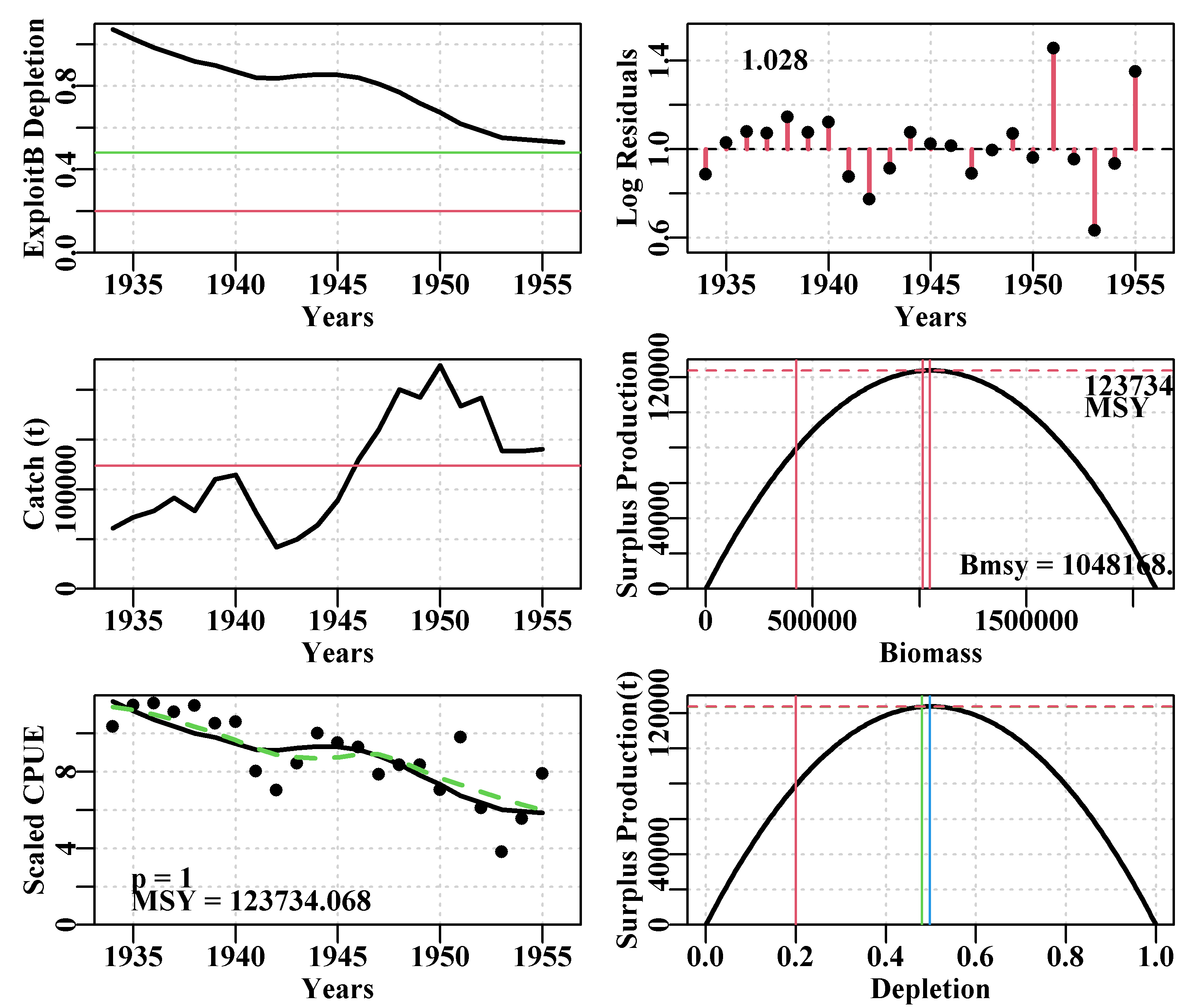
Figure 7.6: A summary of the fit of a surplus production model to the schaef data-set given the optimum parameters from the final nlm() fit. In the CPUE plot, the dashed green line is the simple loess curve fit while the solid red line is the optimal model fit.
The object returned by plotspmmod() is a list of objects containing a collection of results, including the optimum parameters, a matrix (ans$Dynamics$outmat) containing the predicted optimal dynamics, the production curve, and numerous summary results. Once assigned to a particular object in the working environment these can be quickly extracted for use in other functions. Try running str() without the max.level=1 argument or set it = 2, to see more details. Lots of functions generate large, informative objects, you should become familiar with exploring them to make sure you understand what is being produces within different analyses.
 #the high-level structure of ans; try str(ans$Dynamics)
str(ans, width=65, strict.width="cut",max.level=1)
# List of 12
# $ Dynamics :List of 5
# $ BiomProd : num [1:200, 1:2] 100 10687 21273 31860 42446 ...
# ..- attr(*, "dimnames")=List of 2
# $ rmseresid: num 1.03
# $ MSY : num 123731
# $ Bmsy : num 1048169
# $ Dmsy : num 0.498
# $ Blim : num 423562
# $ Btarg : num 1016409
# $ Ctarg : num 123581
# $ Dcurr : Named num 0.528
# ..- attr(*, "names")= chr "1956"
# $ rmse :List of 1
# $ sigma : num 0.169There are also a few MQMF functions to assist with pulling out such results or that use the results from plotspmmod() (see summspm() and spmphaseplot()), which is why the function includes the argument plotout = TRUE, so that a plot need not be produced. However, in many cases it can be simpler just to point to the desired object within the high level object (in this case ans). Notice that the \(MSY\) obtained from the generated productivity curve differs by a small amount from that calculated from the optimal parameters. This is because the productivity curve is obtained numerically by calculating the productivity for a vector of different biomass levels. Its resolution is thus limited by the steps used to generate the biomass vector. Its estimate will invariably be slightly smaller than the parameter derived value.
 #compare the parameteric MSY with the numerical MSY
round(ans$Dynamics$sumout,3)
cat("\n Productivity Statistics \n")
summspm(ans) # the q parameter needs more significantr digits
# msy p FinalDepl InitDepl FinalB
# 123734.068 1.000 0.528 1.072 1113328.480
#
# Productivity Statistics
# Index Statistic
# q 1 0.0000
# MSY 2 123731.0026
# Bmsy 3 1048168.8580
# Dmsy 4 0.4975
# Blim 5 423562.1648
# Btarg 6 1016409.1956
# Ctarg 7 123581.3940
# Dcurr 8 0.5284Finally, to simplify the future use of this double model fitting process there is an MQMF function, fitSPM() that implements the procedure. You can either use that (check out its code, etc), or repeat the contents of the raw code whichever you find most convenient.
7.3.2 Is the Analysis Robust?
Despite my dire warnings you may be wondering why we bothered to fit the model twice, with the starting point for the second fit being the estimated optimum from the first. One should always remember that we are using numerical methods when we fit these models. Such methods are not fool-proof and can discover false minima. If there are any interactions or correlations between the model parameters then slightly different combinations can lead to very similar values of negative log-likelihood. The optimum model fit still exhibits three relative large residuals towards the end of the time-series of cpue, Figure(7.6). They do not exhibit any particular pattern so we assume they only represent uncertainty, which should make one question how good a model fit one has and how reliable the output statistics are from the analysis. One way we can examine the robustness of the model fit is by examining the influence of the initial model parameters on that model fit.
One implementation of a robustness test uses the robustSPM() MQMF function. This generates \(N\) random starting values by using the optimum log-scale parameter values as the respective mean values of some normal random variables with their respective standard deviation values obtained by dividing those mean values by the scaler argument value (see the code and help of robustSPM() for the full details). The object output from robustSPM() includes the \(N\) vectors of randomly varying initial parameter values, which permits their variation to be illustrated and characterized. Of course, as a divisor, the smaller the scaler value the more variable the initial parameter vectors are likely to be and the more often one might expect the model fitting to fail to find the minimum.
 #conduct a robustness test on the Schaefer model fit
data(schaef); schaef <- as.matrix(schaef); reps <- 12
param <- log(c(r=0.15,K=2250000,Binit=2250000,sigma=0.5))
ansS <- fitSPM(pars=param,fish=schaef,schaefer=TRUE,    #use
               maxiter=1000,funk=simpspm,funkone=FALSE) #fitSPM
 #getseed() #generates random seed for repeatable results
set.seed(777852) #sets random number generator with a known seed
robout <- robustSPM(inpar=ansS$estimate,fish=schaef,N=reps,
                    scaler=40,verbose=FALSE,schaefer=TRUE,
                    funk=simpspm,funkone=FALSE)
 #use str(robout) to see the components included in the output
By using the set.seed function the outcome of the pseudo-random numbers used to generate the scattered initial parameter vectors are repeatable. In Table(7.2) we can see that out of 12 trials we obtained 12 with the same final negative log-likelihood to five decimal places, although there was some slight variation apparent in the actual \(r\), \(K\), and \(B_{init}\) values and that led to minor variation in the estimated \(MSY\) values. If we increase the number of trials we finally see some that differ slightly from the optimum.
| ir | iK | iBinit | isigma | iLike | |
|---|---|---|---|---|---|
| 6 | 0.232 | 2521208 | 2394188 | 0.1727 | -5.765 |
| 10 | 0.242 | 2564306 | 1386181 | 0.1659 | 14.306 |
| 11 | 0.237 | 2189281 | 2032237 | 0.1811 | -7.025 |
| 1 | 0.239 | 2351319 | 3401753 | 0.1692 | -6.351 |
| 8 | 0.244 | 2201215 | 2934055 | 0.1795 | -7.078 |
| 3 | 0.233 | 3164529 | 1632687 | 0.1702 | 22.093 |
| 4 | 0.233 | 3482370 | 1584633 | 0.1683 | 34.534 |
| 12 | 0.237 | 3492106 | 1895315 | 0.1653 | 23.789 |
| 2 | 0.247 | 2359029 | 2137751 | 0.1787 | -5.575 |
| 5 | 0.234 | 3057512 | 1502916 | 0.1713 | 23.720 |
| 7 | 0.242 | 1671149 | 2512111 | 0.1687 | 4.228 |
| 9 | 0.230 | 1391893 | 1753155 | 0.1754 | 138.808 |
| r | K | Binit | sigma | -veLL | MSY | |
|---|---|---|---|---|---|---|
| 6 | 0.235 | 2107069 | 2258144 | 0.1687 | -7.93406 | 123725 |
| 10 | 0.235 | 2107034 | 2258103 | 0.1687 | -7.93406 | 123726 |
| 11 | 0.235 | 2107243 | 2258322 | 0.1687 | -7.93406 | 123717 |
| 1 | 0.235 | 2107178 | 2258293 | 0.1687 | -7.93406 | 123722 |
| 8 | 0.235 | 2107119 | 2258218 | 0.1687 | -7.93406 | 123720 |
| 3 | 0.235 | 2107386 | 2258484 | 0.1687 | -7.93406 | 123713 |
| 4 | 0.235 | 2107405 | 2258514 | 0.1687 | -7.93406 | 123713 |
| 12 | 0.235 | 2107417 | 2258533 | 0.1687 | -7.93406 | 123713 |
| 2 | 0.235 | 2106866 | 2257912 | 0.1687 | -7.93406 | 123728 |
| 5 | 0.235 | 2107294 | 2258319 | 0.1687 | -7.93406 | 123713 |
| 7 | 0.235 | 2107319 | 2258401 | 0.1687 | -7.93406 | 123712 |
| 9 | 0.235 | 2106435 | 2257279 | 0.1687 | -7.93406 | 123739 |
Normally one would try more than 12 trials and would examine the effect of the scaler argument. So we will now repeat that analysis 100 times using the same optimum fit and random seed. The table of results output by robustSPM() is sorted by the final -ve log-likelihood but even where this is the same to five decimal places notice there is slight variation in the parameter estimates. This is merely a reflection of using numerical methods.
 #Repeat robustness test on fit to schaef data 100 times
set.seed(777854)
robout2 <- robustSPM(inpar=ansS$estimate,fish=schaef,N=100,
                     scaler=25,verbose=FALSE,schaefer=TRUE,
                     funk=simpspm,funkone=TRUE,steptol=1e-06)
lastbits <- tail(robout2$results[,6:11],10) | r | K | Binit | sigma | -veLL | MSY | |
|---|---|---|---|---|---|---|
| 12 | 0.23513 | 2105553 | 2256358 | 0.1687 | -7.93405 | 123770 |
| 65 | 0.23513 | 2105553 | 2256358 | 0.1687 | -7.93405 | 123770 |
| 47 | 0.23513 | 2105553 | 2256358 | 0.1687 | -7.93405 | 123770 |
| 11 | 0.23513 | 2105553 | 2256358 | 0.1687 | -7.93405 | 123770 |
| 76 | 0.23513 | 2105553 | 2256358 | 0.1687 | -7.93405 | 123770 |
| 57 | 0.23513 | 2105553 | 2256358 | 0.1687 | -7.93405 | 123770 |
| 23 | 0.23513 | 2105553 | 2256358 | 0.1687 | -7.93405 | 123770 |
| 9 | 0.23513 | 2105553 | 2256358 | 0.1687 | -7.93405 | 123770 |
| 93 | 0.23514 | 2105527 | 2256328 | 0.1687 | -7.93405 | 123771 |
| 55 | 0.23514 | 2105510 | 2256327 | 0.1687 | -7.93405 | 123772 |
Table(7.3) is only the bottom 10 records of the sorted 100 replicates, and this indicates that all replicates had the same negative log-likelihood (to 5 decimal places). Again, if you look closely at the values given for r, K, Binit, and MSY you will notice differences. If we plot up the final fitted parameter values as distributions, the scale of the variation becomes clear, Figure(7.7).
 # replicates from the robustness test        Fig 7.7
result <- robout2$results
parset(plots=c(2,2),margin=c(0.35,0.45,0.05,0.05))
hist(result[,"r"],breaks=15,col=2,main="",xlab="r")
hist(result[,"K"],breaks=15,col=2,main="",xlab="K")
hist(result[,"Binit"],breaks=15,col=2,main="",xlab="Binit")
hist(result[,"MSY"],breaks=15,col=2,main="",xlab="MSY") 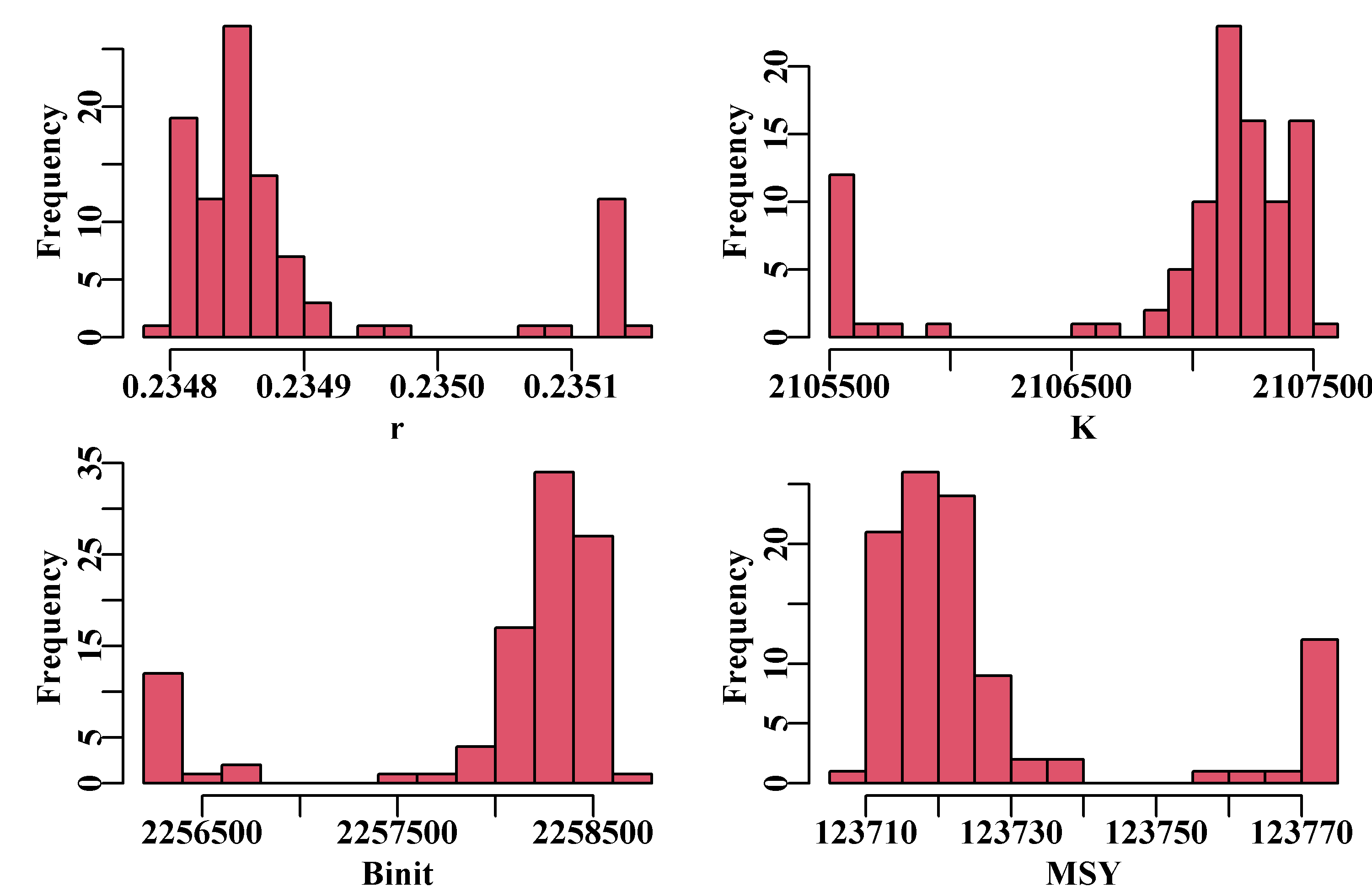
Figure 7.7: Histograms of the main parameters and MSY from the 100 trials in a robustness test of the model fit to the schaef data-set. The parameter estimates are all close, but still there is variation, which is a reflection of estimation uncertainty. To improve on this, one might try a smaller steptol, which defaults to 1e-06, but stable solutions might not always be possible. If you use steptol = 1e-07 the range of values across the variation becomes much tighter but some slight variation remains, as expected when using numerical methods. This is another reason why the particular values for the parameter estimates are most meaningful when we also have an estimate of variation or of uncertainty.
Even with negative log-likelihood values that are very close in value (to five decimal places), Figure(7.7), there are slight deviations possible from the optimum values that occur most often. This emphasizes the need to examine the uncertainty in the analysis closely. Given that most of the trials lead to the same optimum values the median values across all trials can identify optimum values.
An alternative way of visualizing the final variation in parameter estimates from the robustness test is to plot each parameter and model output against each other using the R function pairs(), Figure(7.8), which illustrates the strong correlations between parameters.
 #robustSPM parameters against each other  Fig 7.8
pairs(result[,c("r","K","Binit","MSY")],upper.panel=NULL,pch=1) 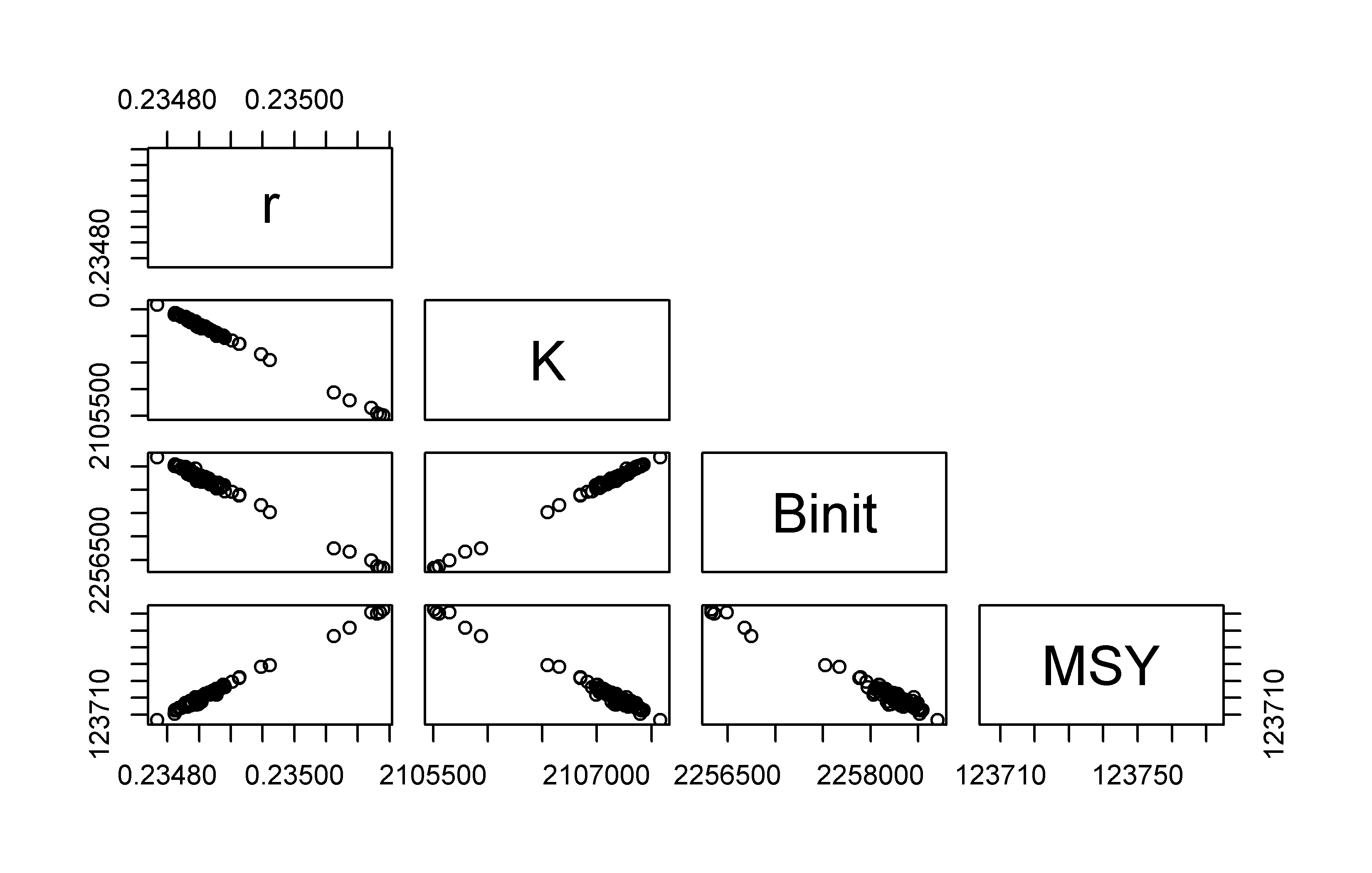
Figure 7.8: Plots of the relationships between parameters in the 100 optimum solutions stemming from fitting a surplus production model to the schaef data-set. The correlation between parameters is clear, although it needs emphasis that the proportional difference between estimates is very small being of the order of 0.2 - 0.3%.
7.3.3 Using Different Data?
The schaef data-set leads to a relatively robust outcome. Before moving on it would be enlightening to repeat the analysis using the dataspm data-set, which leads to more variable outcomes. Hopefully, such findings should encourage any future modellers reading this not to trust the first solution that a numerical optimizer presents.
 #Now use the dataspm data-set, which is noisier
set.seed(777854) #other random seeds give different results
data(dataspm);   fish <- dataspm #to generalize the code
param <- log(c(r=0.24,K=5174,Binit=2846,sigma=0.164))
ans <- fitSPM(pars=param,fish=fish,schaefer=TRUE,maxiter=1000,
             funkone=TRUE)
out <- robustSPM(ans$estimate,fish,N=100,scaler=15, #making
                verbose=FALSE,funkone=TRUE) #scaler=10 gives
result <- tail(out$results[,6:11],10) #16 sub-optimal results | r | K | Binit | sigma | -veLL | MSY | |
|---|---|---|---|---|---|---|
| 46 | 0.2425 | 5171.27 | 2844.29 | 0.1636 | -12.1288 | 313.537 |
| 77 | 0.2425 | 5171.51 | 2843.70 | 0.1636 | -12.1288 | 313.528 |
| 75 | 0.2425 | 5171.81 | 2846.73 | 0.1636 | -12.1288 | 313.545 |
| 79 | 0.2426 | 5169.36 | 2842.83 | 0.1636 | -12.1288 | 313.555 |
| 31 | 3.5610 | 149.62 | 50.74 | 0.2230 | -2.5244 | 133.201 |
| 65 | 0.0321 | 36059.56 | 49.72 | 0.2329 | -1.1783 | 289.163 |
| 60 | 40.3102 | 0.26 | 49.72 | 0.2329 | -1.1783 | 2.592 |
| 57 | 22.1938 | 0.00 | 49.72 | 0.2329 | -1.1783 | 0.016 |
| 38 | 1.1856 | 6062.64 | 49.72 | 0.2329 | -1.1783 | 1797.041 |
| 11 | 0.5954 | 4058.97 | 49.72 | 0.2329 | -1.1783 | 604.180 |
In those bottom six model fits with dataspm we can see cases of very large r values teamed with very small K values, very large K values teamed with small r values, and, in addition, in the last two rows, almost reasonable values for r and K, but very small Binit values.
7.4 Uncertainty
When we tested some model fits for how robust they were to initial conditions we found that when there were multiple parameters being fitted it was possible to obtain essentially the same numerical fit (to a given degree of precision) from slightly different parameter values. While the values did not tend to differ by much, this observation still confirms that when using numerical methods to estimate a set of parameters, the particular parameter values are not the only important outcome. We also need to know how precise those estimates are, we need to know about any uncertainty associated with their estimation. There are a number of approaches one can use to explore the uncertainty within a model fit. Here, using R, we will examine the implementation of four: 1) Likelihood profiles, 2) bootstrap resampling, 3) Asymptotic errors, and 4) Bayesian Posterior Distributions.
7.4.1 Likelihood Profiles
Likelihood profiles do what the name implies and provide insight into how the quality of a model fit might change if the parameters used were slightly different. A model is optimally fitted using maximum likelihood methods (minimization of the -ve log-likelihood), then, while fixing (keeping constant) one or more parameters to pre-determined values, one only fits the remaining unfixed parameters. In this way an optimum fit can be obtained while a given parameter or parameters have been given fixed values. Thus, we can determine how the total likelihood of the model fit will change when selected parameters remain fixed over an array of different values. A worked example should make the process clearer. We can use the abdat data-set, which provides for a reasonable fit to the observed data although leaving a moderate pattern in the residuals for the optimum fit and with relatively large final gradients on the optimum solution (try outfit(ans) to see the results).
 # Fig 7.9 Fit of optimum to the abdat data-set
data(abdat);     fish <- as.matrix(abdat)
colnames(fish) <- tolower(colnames(fish))  # just in case
pars <- log(c(r=0.4,K=9400,Binit=3400,sigma=0.05))
ans <- fitSPM(pars,fish,schaefer=TRUE) #Schaefer
answer <- plotspmmod(ans$estimate,abdat,schaefer=TRUE,addrmse=TRUE) 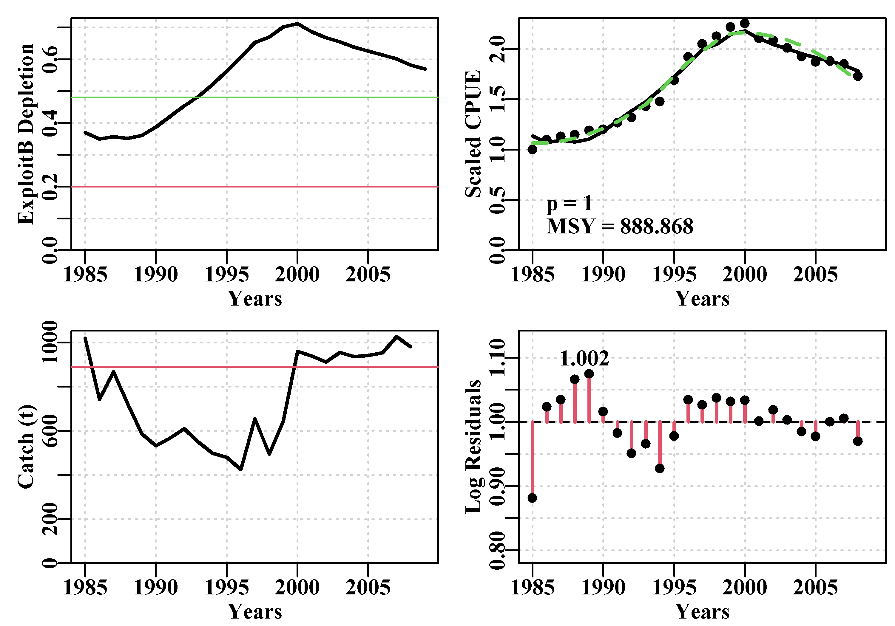
Figure 7.9: Summary plot depicting the fit of the optimum parameters to the abdat data-set. The remaining pattern in the log-normal residuals between the fit and the cpue data are illustrated at the bottom right.
In the chapter On Uncertainty we examined a likelihood profile around a single parameter, here we will explore a little deeper to see some of the issues surrounding the use of likelihood profiles. We already have the optimal fit to the abdat data-set and we can use that as a starting point. If we consider the \(r\) and the \(K\) parameters in turn it becomes more efficient to write a simple function to conduct the profiles in each case to avoid duplicating code. As before we use the negLLP() function to enable some parameters to be fixed while others vary. As seen in the Uncertainty chapter, with one parameter the 95% confidence bounds are approximated by searching for the parameter range that encompasses the minimum log-likelihood plus half the chi-squared value for one degree of freedom (=1.92).
\[\begin{equation} {min(-LL)} + \frac{\chi _{1,1-\alpha }^{2}}{2} \tag{7.17} \end{equation}\]
When plotting each profile we can include this threshold to see where it intersects the likelihood profile, Figure(7.10).
 # likelihood profiles for r and K for fit to abdat  Fig 7.10
 #doprofile input terms are vector of values, fixed parameter
 #location, starting parameters, and free parameter locations.
 #all other input are assumed to be in the calling environment
doprofile <- function(val,loc,startest,indat,notfix=c(2:4)) {
  pname <- c("r","K","Binit","sigma","-veLL")
  numv <- length(val)
  outpar <- matrix(NA,nrow=numv,ncol=5,dimnames=list(val,pname))
  for (i in 1:numv) {  #
    param <- log(startest) # reset the parameters
    param[loc] <- log(val[i]) #insert new fixed value
    parinit <- param   # copy revised parameter vector
    bestmod <- nlm(f=negLLP,p=param,funk=simpspm,initpar=parinit,
                   indat=indat,logobs=log(indat[,"cpue"]),
                   notfixed=notfix)
    outpar[i,] <- c(exp(bestmod$estimate),bestmod$minimum)
  }
  return(outpar)
}
rval <- seq(0.32,0.46,0.001)
outr <- doprofile(rval,loc=1,startest=c(rval[1],11500,5000,0.25),
                  indat=fish,notfix=c(2:4))
Kval <- seq(7200,11500,200)
outk <- doprofile(Kval,loc=2,c(0.4,7200,6500,0.3),indat=fish,
                  notfix=c(1,3,4))
parset(plots=c(2,1),cex=0.85,outmargin=c(0.5,0.5,0,0))
plotprofile(outr,var="r",defpar=FALSE,lwd=2) #MQMF function
plotprofile(outk,var="K",defpar=FALSE,lwd=2) 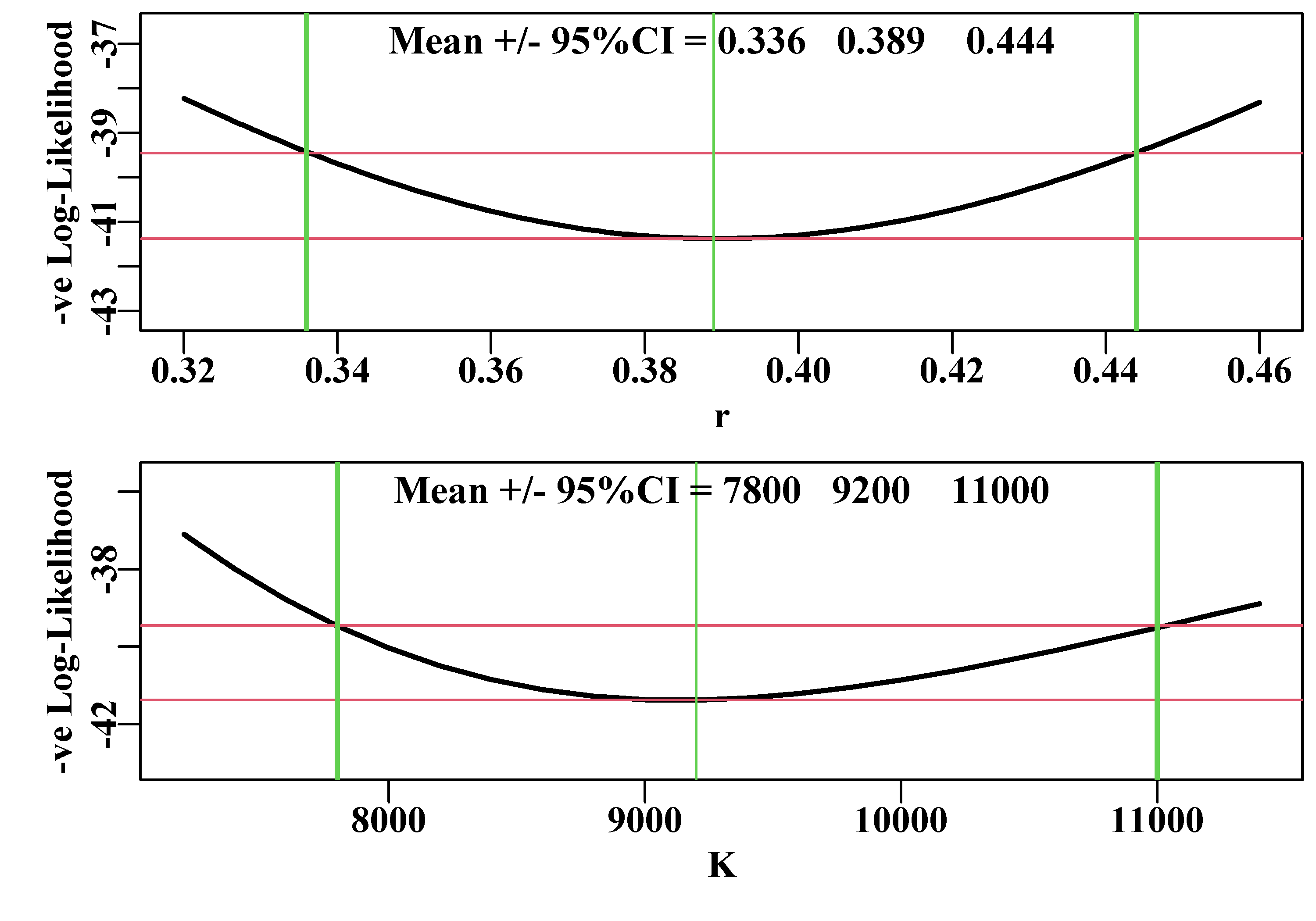
Figure 7.10: Likelihood profiles for both the r and K parameters of the Schaefer model fit to the abdat data-set. The horizontal red lines separate the minimum -veLL from the likelihood value bounding the 95% confidence intervals. The vertical green lines intersect the minimum and the 95% CI. The numbers are the 95% CI surrounding the mean optimum value.
An issue with estimating such confidence bounds is that by only considering single parameters one is ignoring the inter-relationships and correlations between parameters, for which the Schaefer model is well known. But the strong correlation that is expected between the r and K parameters means that a square grid search obtained from combining the two separate individual searches along r and K will lead to many combinations that fall outside of even an approximate fit to the model. It is not impossible to create a two-dimensional likelihood profile (in fact a surface), or indeed a profile across even more parameters, but even two parameters usually requires carefully searching small parts of the surface at a time or other ways of dealing with some of the extremely poor model fits that would be obtained by a simplistic grid search.
Likelihood profiles across single parameters remain useful in situations where a stock assessment has one or more fixed value parameters. This will not happen with such simple models as the Schaefer surplus production model but such situations are not uncommon when dealing with more complex stock assessment models for stocks where biological parameters such as the natural mortality, the steepness of the stock-recruitment curve, and even growth parameters may not be known or are assumed to take the same values as related species. Once an optimum model fit is obtained in an assessment, within which some of the parameters take fixed values, it is possible to re-run the model fit while changing the assumed values for one of the fixed parameters to generate a likelihood profile for that parameter. In that way it is possible to see how consistent the model fit is with regard to the assumed values for the fixed parameters. Generating a likelihood profile in this manner is preferable to merely conducting sensitivity analyses in which we might vary such fixed parameters to a level above and a level below the assumed value to see the effect. Likelihood profiles provide a more detailed exploration of the sensitivity of the modelling to the individual parameters.
With regard to simpler models, such as we are dealing with here, there are other ways of examining the uncertainty inherent in the modelling that can attempt to take into account the correlations between parameters.
7.4.2 Bootstrap Confidence Intervals
One way to characterize uncertainty in a model fit is to generate percentile confidence intervals around parameters and model outputs (MSY, etc) by taking bootstrap samples of the log-normal residuals associated with the cpue and using those to generate new bootstrap cpue samples with which to replace the original cpue time-series (Haddon, 2011). Each time such a bootstrap sample is made, the model is re-fit and the solutions stored for further analysis. To conduct such an analysis on surplus production models one can use the MQMF function spmboot(). Once we have found suitable starting parameters, we can use the fitSPM() function to obtain an optimum fit and it is the log-normal residuals associated with that optimum fit that are bootstrapped. Here we will use the relatively noisy dataspm data-set to illustrate these ideas
 #find optimum Schaefer model fit to dataspm data-set Fig 7.11
data(dataspm)
fish <- as.matrix(dataspm)
colnames(fish) <- tolower(colnames(fish))
pars <- log(c(r=0.25,K=5500,Binit=3000,sigma=0.25))
ans <- fitSPM(pars,fish,schaefer=TRUE,maxiter=1000) #Schaefer
answer <- plotspmmod(ans$estimate,fish,schaefer=TRUE,addrmse=TRUE) 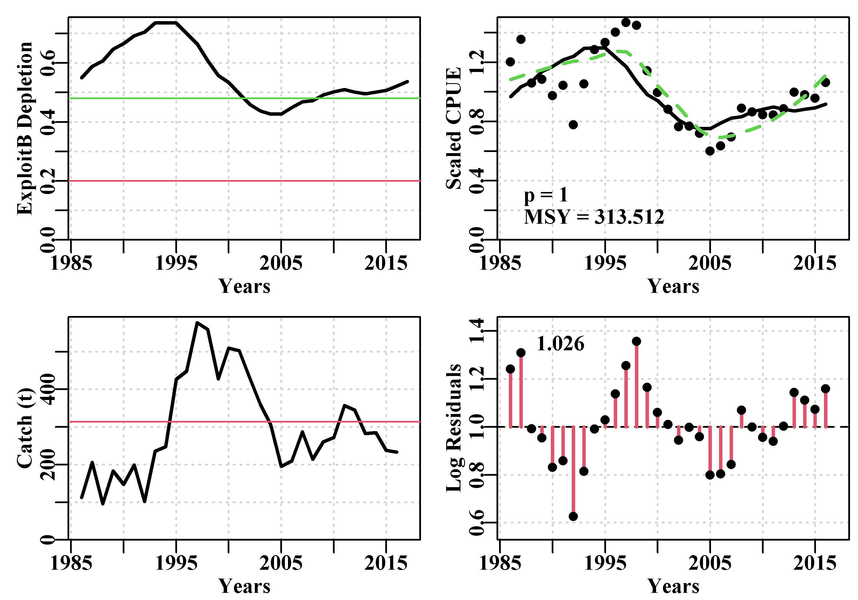
Figure 7.11: Summary plot depicting the fit of the optimum parameters to the dataspm data-set. The log-normal residuals between the fit and the cpue data are illustrated at the bottom right. These are what are bootstrapped and each bootstrap sample multiplied by the optimum predicted cpue time-series to obtain each bootstrap cpue time-series.
Once we have an optimum fit we can proceed to conduct a bootstrap analysis. One would usually run at least 1000 replicates, and often more, even though that might take a few minutes to complete. In this case, even in the optimum fit there is a pattern in the log-normal residuals, suggesting that the model structure is missing some approximately cyclic event affecting the fishery.
 #bootstrap the log-normal residuals from optimum model fit
set.seed(210368)
reps <- 1000 # can take 10 sec on a large Desktop. Be patient
 #startime <- Sys.time()  # schaefer=TRUE is the default
boots <- spmboot(ans$estimate,fishery=fish,iter=reps)
 #print(Sys.time() - startime) # how long did it take?
str(boots,max.level=1)
# List of 2
# $ dynam : num [1:1000, 1:31, 1:5] 2846 3555 2459 3020 1865 ...
# ..- attr(*, "dimnames")=List of 3
# $ bootpar: num [1:1000, 1:8] 0.242 0.236 0.192 0.23 0.361 ...
# ..- attr(*, "dimnames")=List of 2The output contains the dynamics of each run with the predicted model biomass, each bootstrap cpue sample, the predicted cpue for each bootstrap sample, the depletion time-series, and the annual harvest rate time-series (reps=1000 runs for 31 years with 5 variables stored). Each of these can be used to illustrate and summarize the outcomes and uncertainty within the analysis. Given the relatively large residuals in Figure(7.11) one might expect a relatively high degree of uncertainty, Table(7.5).
 #Summarize bootstrapped parameter estimates as quantiles  Table 7.6
bootpar <- boots$bootpar
rows <- colnames(bootpar)
columns <- c(c(0.025,0.05,0.5,0.95,0.975),"Mean")
bootCI <- matrix(NA,nrow=length(rows),ncol=length(columns),
                 dimnames=list(rows,columns))
for (i in 1:length(rows)) {
   tmp <- bootpar[,i]
   qtil <- quantile(tmp,probs=c(0.025,0.05,0.5,0.95,0.975),na.rm=TRUE)
   bootCI[i,] <- c(qtil,mean(tmp,na.rm=TRUE))
} | 0.025 | 0.05 | 0.5 | 0.95 | 0.975 | Mean | |
|---|---|---|---|---|---|---|
| r | 0.1321 | 0.1494 | 0.2458 | 0.3540 | 0.3735 | 0.2484 |
| K | 3676.3569 | 3840.6961 | 5184.2237 | 7965.3318 | 8997.4945 | 5481.5140 |
| Binit | 1727.1976 | 1845.8458 | 2829.0085 | 4935.7516 | 5603.2871 | 3041.6876 |
| sigma | 0.1388 | 0.1423 | 0.1567 | 0.1626 | 0.1630 | 0.1551 |
| -veLL | -17.2319 | -16.4647 | -13.4785 | -12.3160 | -12.2377 | -13.8150 |
| MSY | 280.3701 | 289.4673 | 318.4197 | 352.7195 | 366.2422 | 319.5455 |
| Depl | 0.3384 | 0.3666 | 0.5286 | 0.6693 | 0.6992 | 0.5240 |
| Harv | 0.0508 | 0.0576 | 0.0877 | 0.1161 | 0.1236 | 0.0871 |
Such percentile confidence intervals can be visualized using histograms and including the respective selected percentile CI.
One would expect 1000 replicates would provide for a smooth response and representative confidence bounds but sometimes, especially with noisy data, one needs more replicates to obtain smooth representations of uncertainty. Taking 20 seconds for 2000 replicates might seem like a long time, but considering that such things used to take hours and even days, about 20 seconds is remarkable. Note that the confidence bounds are not necessarily symmetrical around either the mean or the median estimates. Notice also that with the final year depletion estimates the 5th percentile CI is well above \(0.2B_0\), implying that even though this analysis is uncertain the current depletion level is above the default limit reference point for biomass depletion used most everywhere with more than a 95% likelihood. We would need the central 80th percentiles to find the lower 10% bound, but it is bound to be higher than the 5th percentile. The medians and means exhibited by the K and the Binit values differ more than with the other parameters and model outputs, which suggests some evidence of bias, Figure(7.12). Because roughness remains in some plots these would be improved by increasing the number of replicates.
 #boostrap CI. Note use of uphist to expand scale  Fig 7.12
{colf <- c(1,1,1,4); lwdf <- c(1,3,1,3); ltyf <- c(1,1,1,2)
colsf <- c(2,3,4,6)
parset(plots=c(3,2))
hist(bootpar[,"r"],breaks=25,main="",xlab="r")
abline(v=c(bootCI["r",colsf]),col=colf,lwd=lwdf,lty=ltyf)
uphist(bootpar[,"K"],maxval=14000,breaks=25,main="",xlab="K")
abline(v=c(bootCI["K",colsf]),col=colf,lwd=lwdf,lty=ltyf)
hist(bootpar[,"Binit"],breaks=25,main="",xlab="Binit")
abline(v=c(bootCI["Binit",colsf]),col=colf,lwd=lwdf,lty=ltyf)
uphist(bootpar[,"MSY"],breaks=25,main="",xlab="MSY",maxval=450)
abline(v=c(bootCI["MSY",colsf]),col=colf,lwd=lwdf,lty=ltyf)
hist(bootpar[,"Depl"],breaks=25,main="",xlab="Final Depletion")
abline(v=c(bootCI["Depl",colsf]),col=colf,lwd=lwdf,lty=ltyf)
hist(bootpar[,"Harv"],breaks=25,main="",xlab="End Harvest Rate")
abline(v=c(bootCI["Harv",colsf]),col=colf,lwd=lwdf,lty=ltyf) }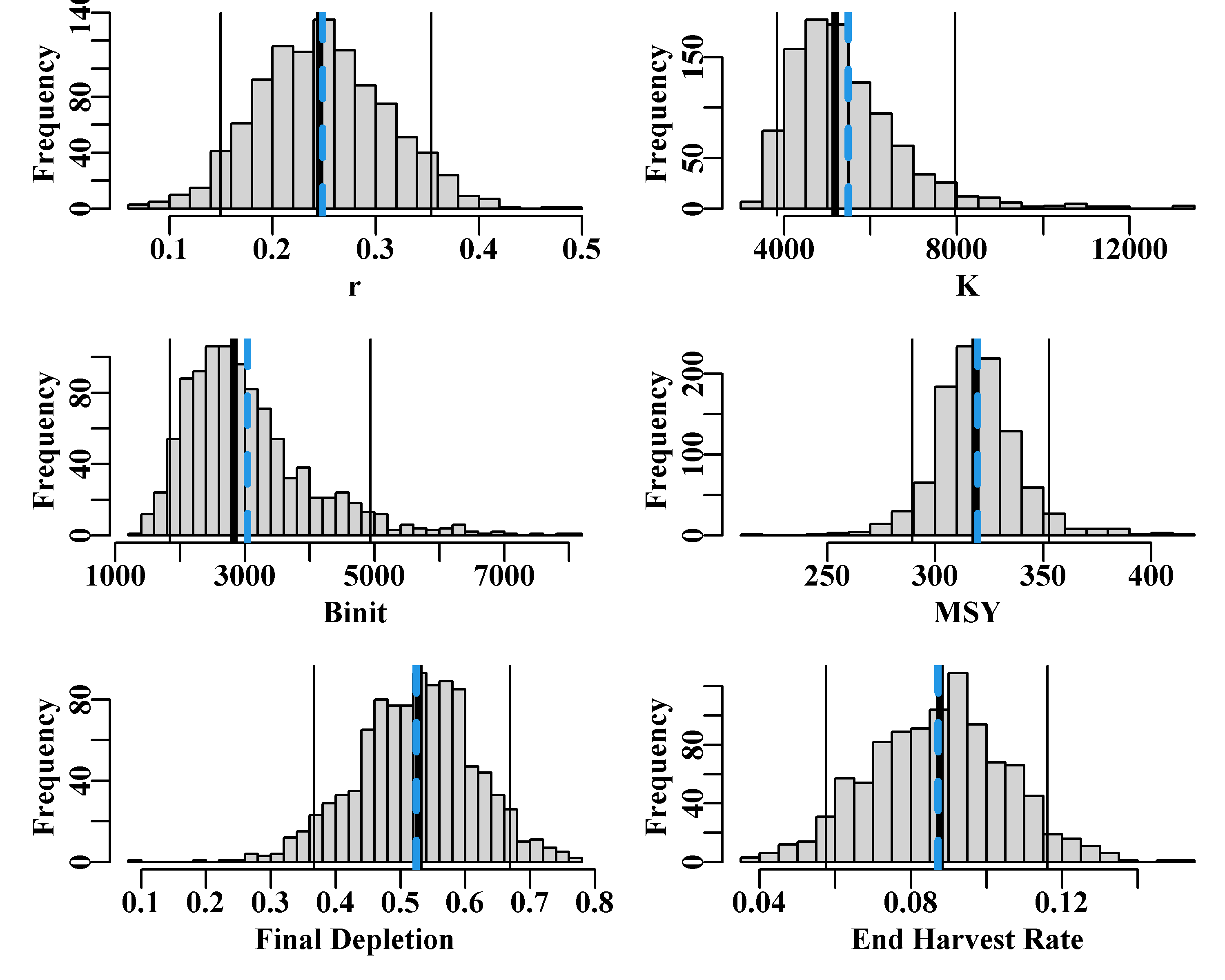
Figure 7.12: The 1000 bootstrap replicates from the optimum spm fit to the dataspm data-set. The vertical lines, in each case, are the median and 90th percentile confidence intervals and the dashed vertical blue lines are the mean values. The function uphist() is used to expand the x-axis in K, Binit, and MSY.
The fitted trajectories, stored in boots$dynam can also provide a visual indication of the uncertainty surrounding the analysis.
 #Fig7.13 1000 bootstrap trajectories for dataspm model fit
dynam <- boots$dynam
years <- fish[,"year"]
nyrs <- length(years)
parset()
ymax <- getmax(c(dynam[,,"predCE"],fish[,"cpue"]))
plot(fish[,"year"],fish[,"cpue"],type="n",ylim=c(0,ymax),
     xlab="Year",ylab="CPUE",yaxs="i",panel.first = grid())
for (i in 1:reps) lines(years,dynam[i,,"predCE"],lwd=1,col=8)
lines(years,answer$Dynamics$outmat[1:nyrs,"predCE"],lwd=2,col=0)
points(years,fish[,"cpue"],cex=1.2,pch=16,col=1)
percs <- apply(dynam[,,"predCE"],2,quants)
arrows(x0=years,y0=percs["5%",],y1=percs["95%",],length=0.03,
angle=90,code=3,col=0) 
Figure 7.13: A plot of the original observed CPUE (black dots), the optimum predicted CPUE (solid line), the 1000 bootstrap predicted CPUE (the grey lines), and the 90th percentile confidence intervals around those predicted values (the vertical bars).
There are clearly some deviations between the predicted and the observed CPUE values Figure(7.13), but the median estimates and the confidence bounds around them remain well defined.
Remember that whenever using a bootstrap on time-series data, where the values at time \(t+1\) are related to the values at time \(t\), it is necessary to bootstrap the residual values from any fitted model and relate them back to the optimum fitted values. With cpue data we are usually using log-normal residual errors so once the optimal solution is found those residual are defined as:
\[\begin{equation} \hat{I}_{t,resid} = \frac{I_t}{\hat{I_t}} \tag{7.18} \end{equation}\]
where \(I_t\) is the observed cpue in year \(t\), \({I_t}/{\hat{I_t}}\) is the observed divided by the predicted cpue in year \(t\) (the log-normal residual \(\hat{I}_{t,resid}\). There will be a time-series of such residuals and the bootstrap generation consists of randomly selecting values from the time-series, with replacement, so that a bootstrap sample of log-normal residuals is prepared. These are then multiplied by the original optimal predicted cpue values to generate different time-series of bootstrapped cpue.
\[\begin{equation} {I_t}^* = \hat{I_t} * \left [ \frac{I}{\hat{I}} \right ]^* \tag{7.19} \end{equation}\]
where the superscript \(*\) denotes a bootstrap sample, with \({I_t}^*\) denoting the bootstrap cpue sample for year \(t\), the \(\left [ \frac{I}{\hat{I}} \right ]^*\) denotes a single random sample from the log-normal residuals, which is then multiplied by the year’s predicted cpue. These equations reflect particular lines of code within the MQMF function spmboot().
A worthwhile exercise would be to repeat this analysis but everywhere schaefer = TRUE replace that with FALSE so as to fit the model using the Fox surplus production model. Then it would be possible to compare the uncertainty of the two models.
 #Fit the Fox model to dataspm; note different parameters
pars <- log(c(r=0.15,K=6500,Binit=3000,sigma=0.20))
ansF <- fitSPM(pars,fish,schaefer=FALSE,maxiter=1000) #Fox version
bootsF <- spmboot(ansF$estimate,fishery=fish,iter=reps,schaefer=FALSE)
dynamF <- bootsF$dynam
# bootstrap trajectories from both model fits Fig 7.14
parset()
ymax <- getmax(c(dynam[,,"predCE"],fish[,"cpue"]))
plot(fish[,"year"],fish[,"cpue"],type="n",ylim=c(0,ymax),
xlab="Year",ylab="CPUE",yaxs="i",panel.first = grid())
for (i in 1:reps) lines(years,dynamF[i,,"predCE"],lwd=1,col=1,lty=1)
for (i in 1:reps) lines(years,dynam[i,,"predCE"],lwd=1,col=8)
lines(years,answer$Dynamics$outmat[1:nyrs,"predCE"],lwd=2,col=0)
points(years,fish[,"cpue"],cex=1.1,pch=16,col=1)
percs <- apply(dynam[,,"predCE"],2,quants)
arrows(x0=years,y0=percs["5%",],y1=percs["95%",],length=0.03,
angle=90,code=3,col=0)
legend(1985,0.35,c("Schaefer","Fox"),col=c(8,1),bty="n",lwd=3) 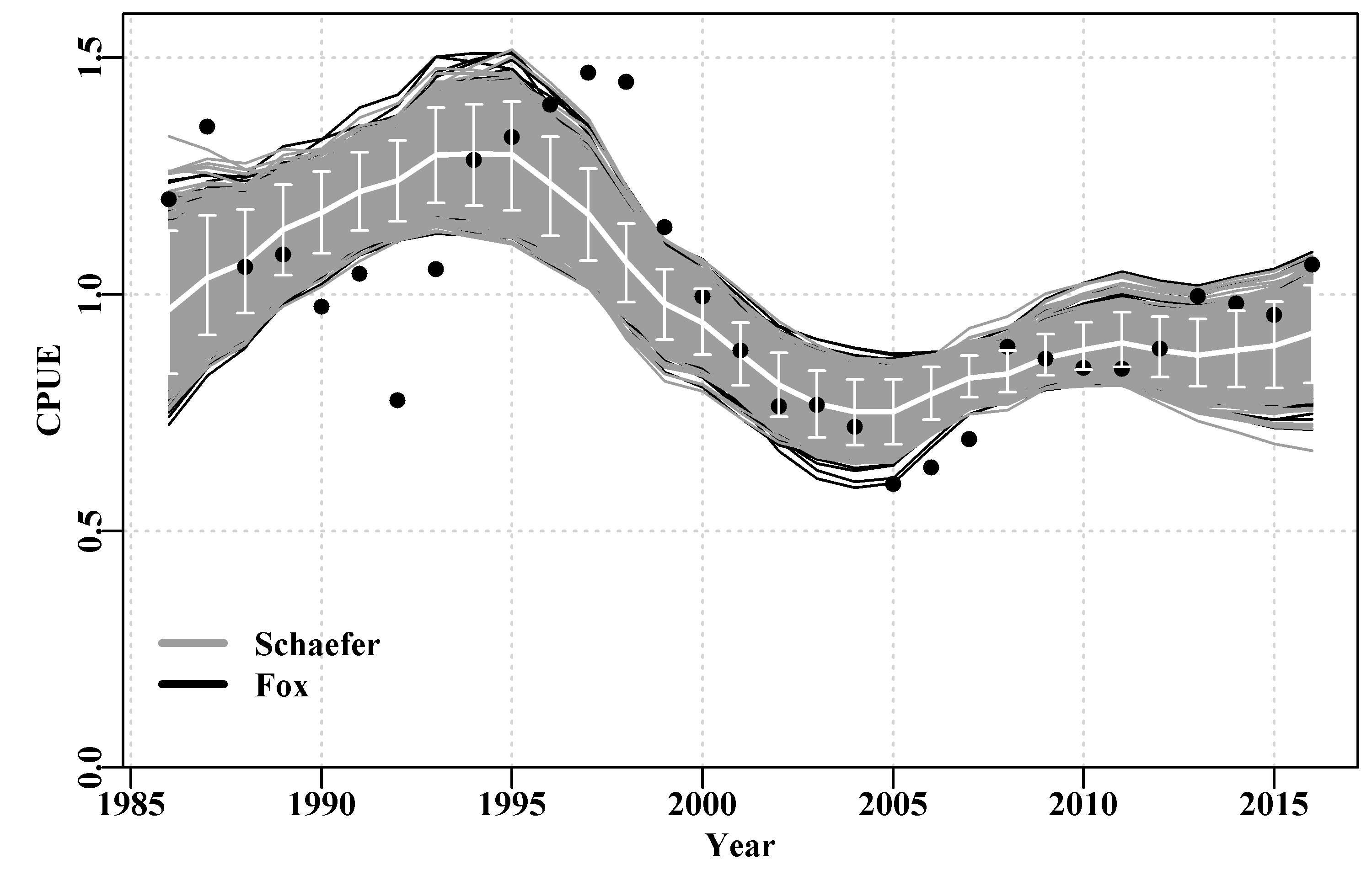
Figure 7.14: A plot of the original observed CPUE (dots), the optimum predicted CPUE (solid white line) with the 90th percentile confidence intervals (the white bars). The black lines are the Fox model bootstrap replicates while the grey lines over the black are those from the Schaefer model.
It could be argued that the Fox model is more successful at capturing the variability in this data as the spread of the black lines is slightly greater than that of the grey, Figure(7.14). Alternatively, it could be argued that the Fox model is less certain. Overall there is not a lot of difference between the outputs of the Schaefer and Fox models as even their predicted \(MSY\) values are very similar (313.512t vs 311.661t). However, in the end it appears the non-linearity in the density-dependence within the Fox model gives it more flexibility and hence it is able to capture the variability of the original data slightly better than the more rigid Schaefer model (hence its slighter smaller -ve log-likelihood, see outfit(ansF)). But neither model can capture the cyclic property exhibited in the residuals, which implies there is some process not being included in the modelled dynamics, a model misspecification. Neither model is completely adequate although either may provide a sufficient approximation to the dynamics that they could be used to generate management advice (with caveats about the cyclic process remaining the same through time, etc).
7.4.3 Parameter Correlations
The combined bootstrap samples and associated estimates provide a characterization of the variability across the parameters reflecting both the data and the model being fitted. If we plot the various parameters against each other any parameter correlations become apparent. The strong negative curvi-linear relationship between \(r\) and \(K\) is very apparent, while the relationships with and between the other parameters are also neither random nor smoothly normal. There are some points at extreme values but they remain rare, nevertheless, the plots do illustrate the form of the variation within this analysis.
 # plot variables against each other, use MQMF panel.cor  Fig 7.15
pairs(boots$bootpar[,c(1:4,6,7)],lower.panel=panel.smooth,
upper.panel=panel.cor,gap=0,lwd=2,cex=0.5) 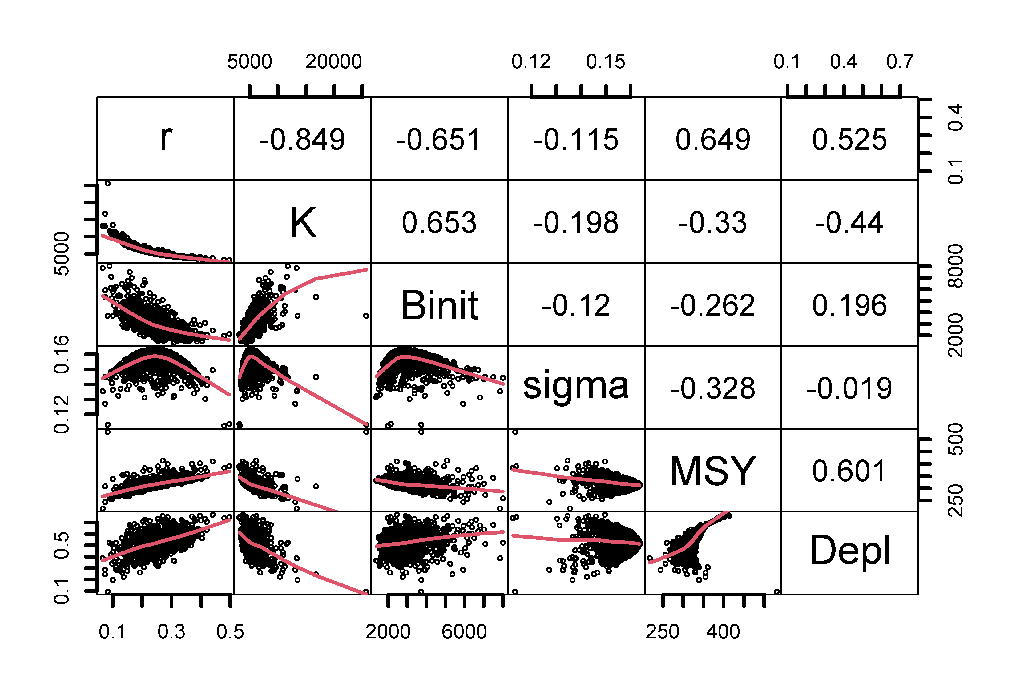
Figure 7.15: The relationships between the model parameters and some outputs for the Schaefer model (use bootsF$bootpar for the Fox model ). The lower panels have a red smoother line through the data illustrating any trends, while the upper panels have the linear correlation coefficient. The few extreme values distort the plots.
7.4.4 Asymptotic Errors
As described in the chapter On Uncertainty, a classical method of characterizing the uncertainty associated with the parameter estimates in a model fitting exercise is to use what are known as asymptotic errors. These derive from the variance-covariance matrix that can be used to describe the variability and interactions between the parameters of a model. In the section on the bootstrap it was possible to visualize the relationships between the parameters using the pairs() function and they were clearly not nicely multi-variate normal. Nevertheless, it remains possible to use the multi-variate normal derived from the variance-covariance matrix (vcov) to characterize a model’s uncertainty. We can estimate the vcov as an option when fitting a model using either optim() or nlm().
 #Start the SPM analysis using asymptotic errors.
data(dataspm)    # Note the use of hess=TRUE in call to fitSPM
fish <- as.matrix(dataspm)     # using as.matrix for more speed
colnames(fish) <- tolower(colnames(fish))  # just in case
pars <- log(c(r=0.25,K=5200,Binit=2900,sigma=0.20))
ans <- fitSPM(pars,fish,schaefer=TRUE,maxiter=1000,hess=TRUE)
We can see the outcome from fitting the Schaefer surplus production model to the dataspm data-set with the hess argument set to TRUE by using the outfit() function.
# nlm solution:
# minimum     :  -12.12879
# iterations  :  2
# code        :  2 >1 iterates in tolerance, probably solution
#         par      gradient   transpar
# 1 -1.417080  0.0031126661    0.24242
# 2  8.551232 -0.0017992364 5173.12308
# 3  7.953564 -0.0009892147 2845.69834
# 4 -1.810225 -0.0021756288    0.16362
# hessian     :
#              [,1]        [,2]          [,3]        [,4]
# [1,] 1338.3568627 1648.147068  -74.39814471 -0.14039276
# [2,] 1648.1470677 2076.777078 -115.32342460 -1.80063349
# [3,]  -74.3981447 -115.323425   25.48912486 -0.01822396
# [4,]   -0.1403928   -1.800633   -0.01822396 61.99195077
The final minimization within fitSPM() uses maximum likelihood methods (actually the minimum negative log-likelihood) and so we need to invert the Hessian to obtain the variance-covariance matrix. The square-root of the diagonal also gives estimates of the standard error for each parameter (see chapter On Uncertainty).
 #calculate the var-covar matrix and the st errors
vcov <- solve(ans$hessian) # calculate variance-covariance matrix
label <- c("r","K", "Binit","sigma")
colnames(vcov) <- label; rownames(vcov) <- label
outvcov <- rbind(vcov,sqrt(diag(vcov)))
rownames(outvcov) <- c(label,"StErr") | r | K | Binit | sigma | |
|---|---|---|---|---|
| r | 0.06676 | -0.05631 | -0.05991 | -0.00150 |
| K | -0.05631 | 0.04814 | 0.05344 | 0.00129 |
| Binit | -0.05991 | 0.05344 | 0.10615 | 0.00145 |
| sigma | -0.00150 | 0.00129 | 0.00145 | 0.01617 |
| StErr | 0.25838 | 0.21940 | 0.32581 | 0.12714 |
Now that we have the optimum solution and the variance-covariance matrix we can use a multi-variate Normal distribution to provide the basis for obtaining multiple plausible combinations of parameters which can be used to calculate outputs such as the \(MSY\), as well as describe the expected dynamics. Base R does not include methods for sampling from a multi-variate normal distribution but there are freely available packages that do. We will use the mvtnorm package downloadable from CRAN. When using such a package one can determine who wrote it and other important information by using the packageDescription() function. Alternatively, by examining one of the help files for a function within the package, if you scroll to the bottom of the page and click the Index hyperlink, this will enables you to read the DESCRIPTION file directly.
 #generate 1000 parameter vectors from multi-variate normal
library(mvtnorm)   # use RStudio, or install.packages("mvtnorm")
N <- 1000 # number of parameter vectors, use vcov from above
mvn <- length(fish[,"year"]) #matrix to store cpue trajectories
mvncpue <- matrix(0,nrow=N,ncol=mvn,dimnames=list(1:N,fish[,"year"]))
columns <- c("r","K","Binit","sigma")
optpar <- ans$estimate # Fill matrix with mvn parameter vectors
mvnpar <- matrix(exp(rmvnorm(N,mean=optpar,sigma=vcov)),nrow=N,
                 ncol=4,dimnames=list(1:N,columns))
msy <- mvnpar[,"r"]*mvnpar[,"K"]/4
nyr <- length(fish[,"year"])
depletion <- numeric(N) #now calculate N cpue series in linear space
for (i in 1:N) { # calculate dynamics for each parameter set
  dynamA <- spm(log(mvnpar[i,1:4]),fish)
  mvncpue[i,] <- dynamA$outmat[1:nyr,"predCE"]
  depletion[i] <- dynamA$outmat["2016","Depletion"]
}
mvnpar <- cbind(mvnpar,msy,depletion) # try head(mvnpar,10)
With the bootstraps, when the implied CPUE trajectories are plotted, Figures(7.13) and (7.14), the outcome appears plausible. On the other hand, with the asymptotic errors, when we plot the implied dynamics, Figure(7.16), a proportion, admittedly falling outside the 90th percentile confidence intervals, which are themselves wildly asymmetric, generate wildly fluctuating dynamics, which can even imply the stock goes extinct.
 #data and trajectories from 1000 MVN parameter vectors   Fig 7.16
plot1(fish[,"year"],fish[,"cpue"],type="p",xlab="Year",ylab="CPUE",
      maxy=2.0)
for (i in 1:N) lines(fish[,"year"],mvncpue[i,],col="grey",lwd=1)
points(fish[,"year"],fish[,"cpue"],pch=1,cex=1.3,col=1,lwd=2) # data
lines(fish[,"year"],exp(simpspm(optpar,fish)),lwd=2,col=1)# pred
percs <- apply(mvncpue,2,quants)  # obtain the quantiles
arrows(x0=fish[,"year"],y0=percs["5%",],y1=percs["95%",],length=0.03,
       angle=90,code=3,col=1) #add 90% quantiles
msy <- mvnpar[,"r"]*mvnpar[,"K"]/4  # 1000 MSY estimates
text(2010,1.75,paste0("MSY ",round(mean(msy),3)),cex=1.25,font=7) 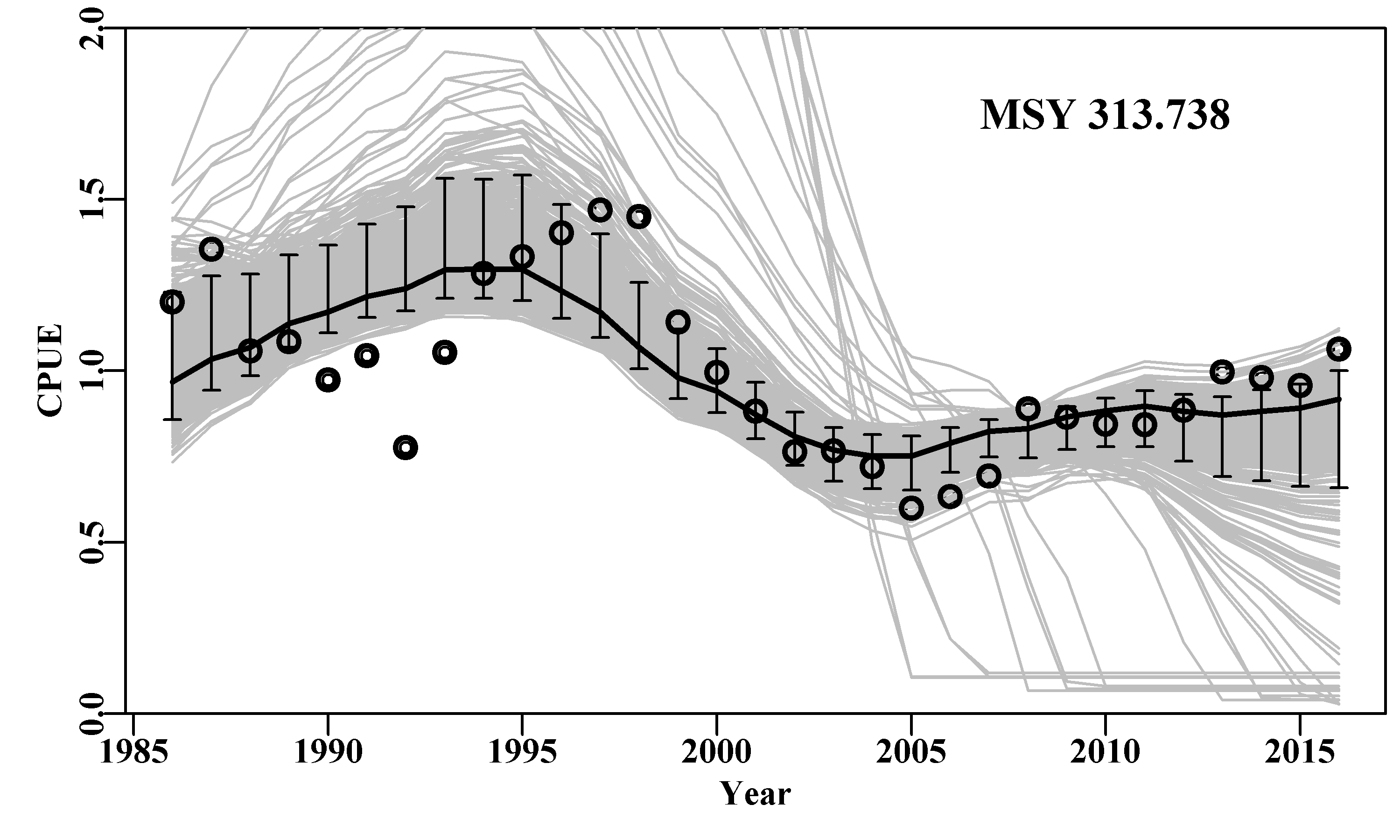
Figure 7.16: The 1000 predicted cpue trajectories derived from random parameter vectors sampled from the multi-variate normal distribution defined by the optimum parameters and their related variance-covariance matrix.
The mean \(MSY\) estimate from the use of asymptotic errors is very similar to that produced by the bootstrapped estimate (319.546, Table(7.5)), and the 90th quantile confidence bounds appear meaningful, although far more skewed than in the bootstrap analysis. However, it is clear that the use of the multi-variate normal distribution can lead to some rather implausible parameter combinations that, in turn, lead to implausible cpue trajectories, which deviate very far from the observed cpue. This does not mean that asymptotic errors should not be used, but rather if one does use them then their implications should be examined for plausibility.
In this case we can search for the parameter combinations that led to the extreme results by finding those records where the final cpue level was < 0.4.
 #Isolate errant cpue trajectories Fig 7.17
pickd <- which(mvncpue[,"2016"] < 0.40)
plot1(fish[,"year"],fish[,"cpue"],type="n",xlab="Year",ylab="CPUE",
      maxy=6.25)
for (i in 1:length(pickd))
  lines(fish[,"year"],mvncpue[pickd[i],],col=1,lwd=1)
points(fish[,"year"],fish[,"cpue"],pch=16,cex=1.25,col=4)
lines(fish[,"year"],exp(simpspm(optpar,fish)),lwd=3,col=2,lty=2) 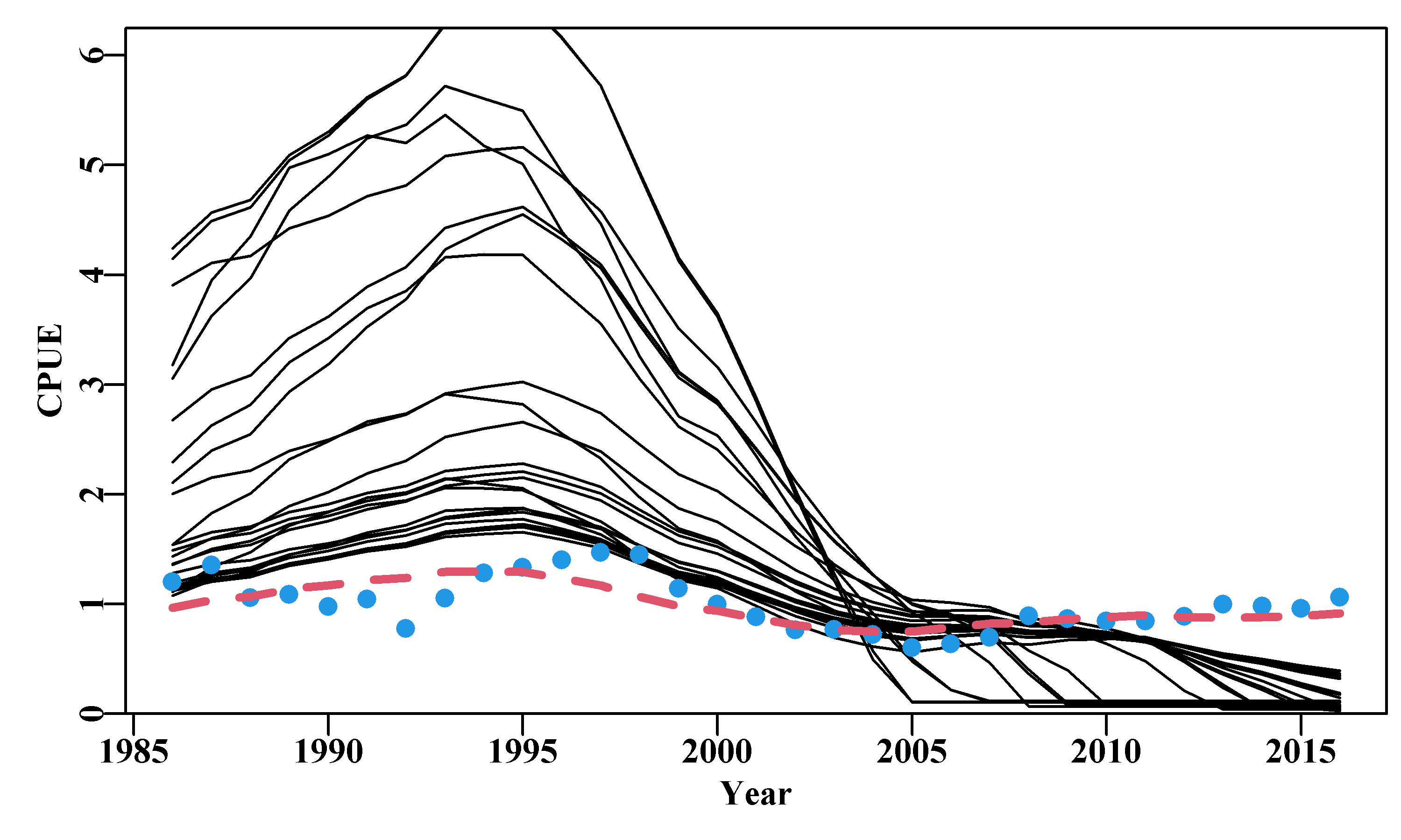
Figure 7.17: The 34 asymptotic error cpue trajectories that were predicted to have a cpue < 0.4 in 2016. The dots are the original data and the dashed line the optimum model fit.
Now we have identified the majority of the errant trajectories, with their respective parameter vectors we can compare what we take to be the non-errant trajectories by plotting them in a manner so we can identify who is who, Figure(7.18).
 #Use adhoc function to plot errant parameters Fig 7.18
parset(plots=c(2,2),cex=0.85)
outplot <- function(var1,var2,pickdev) {
  plot1(mvnpar[,var1],mvnpar[,var2],type="p",pch=16,cex=1.0,
        defpar=FALSE,xlab=var1,ylab=var2,col=8)
  points(mvnpar[pickdev,var1],mvnpar[pickdev,var2],pch=16,cex=1.0)
}
outplot("r","K",pickd) # assumes mvnpar in working environment
outplot("sigma","Binit",pickd)
outplot("r","Binit",pickd)
outplot("K","Binit",pickd) 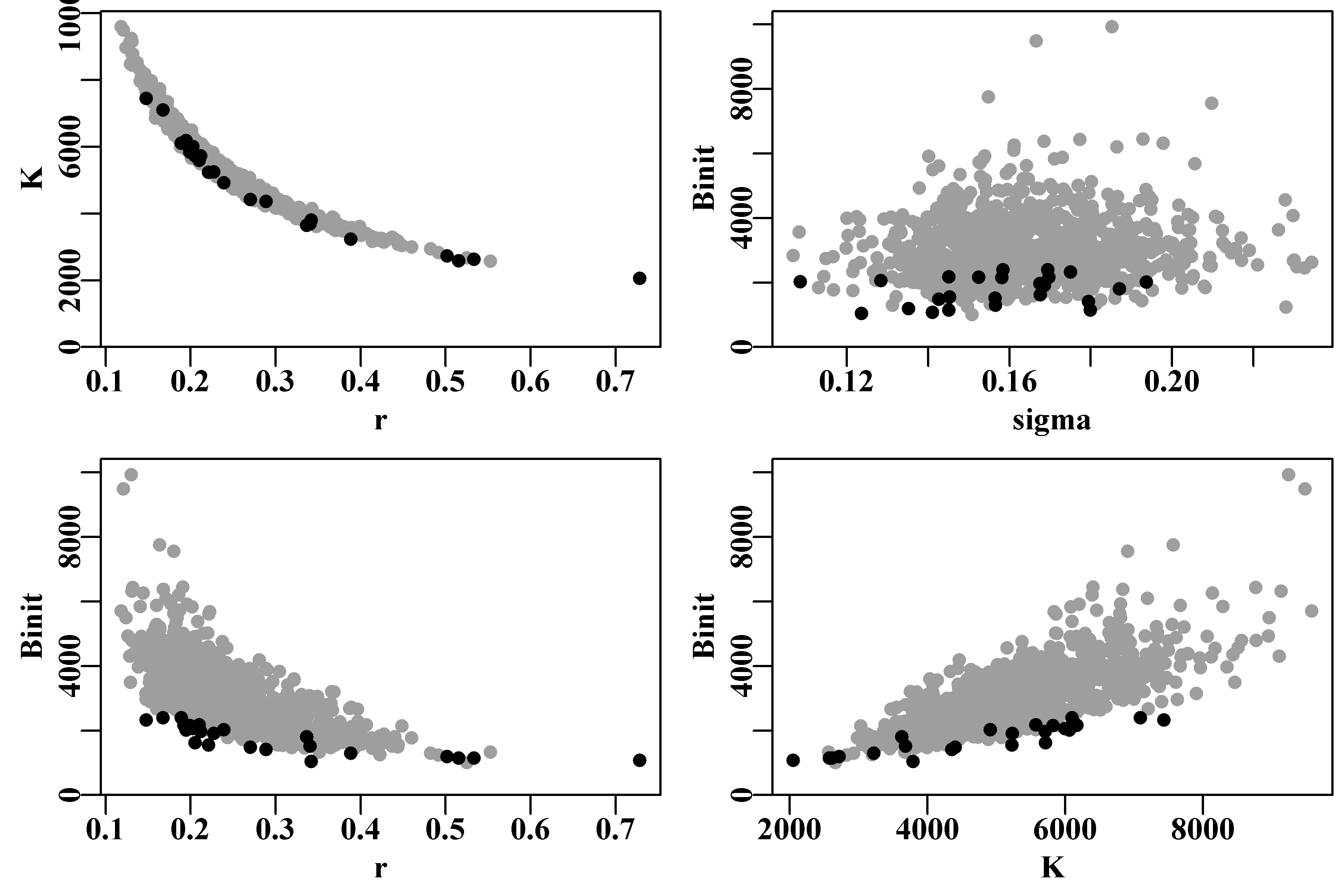
Figure 7.18: The spread of parameter values from the asymptotic error samples with the values that predicted final cpue < 0.4 highlighted in black. It appears that low values of Binit are mostly behind the implausible trajectories.
When we plot the model variables against each other, Figure(7.19), the lack of a relationship between \(sigma\) and the other parameters is expected for Normally or multi-variate Normally distributed variables. However, this differs markedly from the relationship obtained from the bootstrap samples, Figure(7.15). In addition, the relationships between the three main parameters \(r\), \(K\), and \(B_{init}\) are far smoother than was seen in the bootstrap sampling. To our eyes such symmetry and cleanliness of bounds appears more acceptable than the relationships seen in the bootstrap samples, Figure(7.19). Nevertheless, the plots of depletion indicate some trajectories appear to have gone extinct.
 #asymptotically sampled parameter vectors  Fig 7.19
pairs(mvnpar,lower.panel=panel.smooth, upper.panel=panel.cor,
gap=0,cex=0.25,lwd=2) 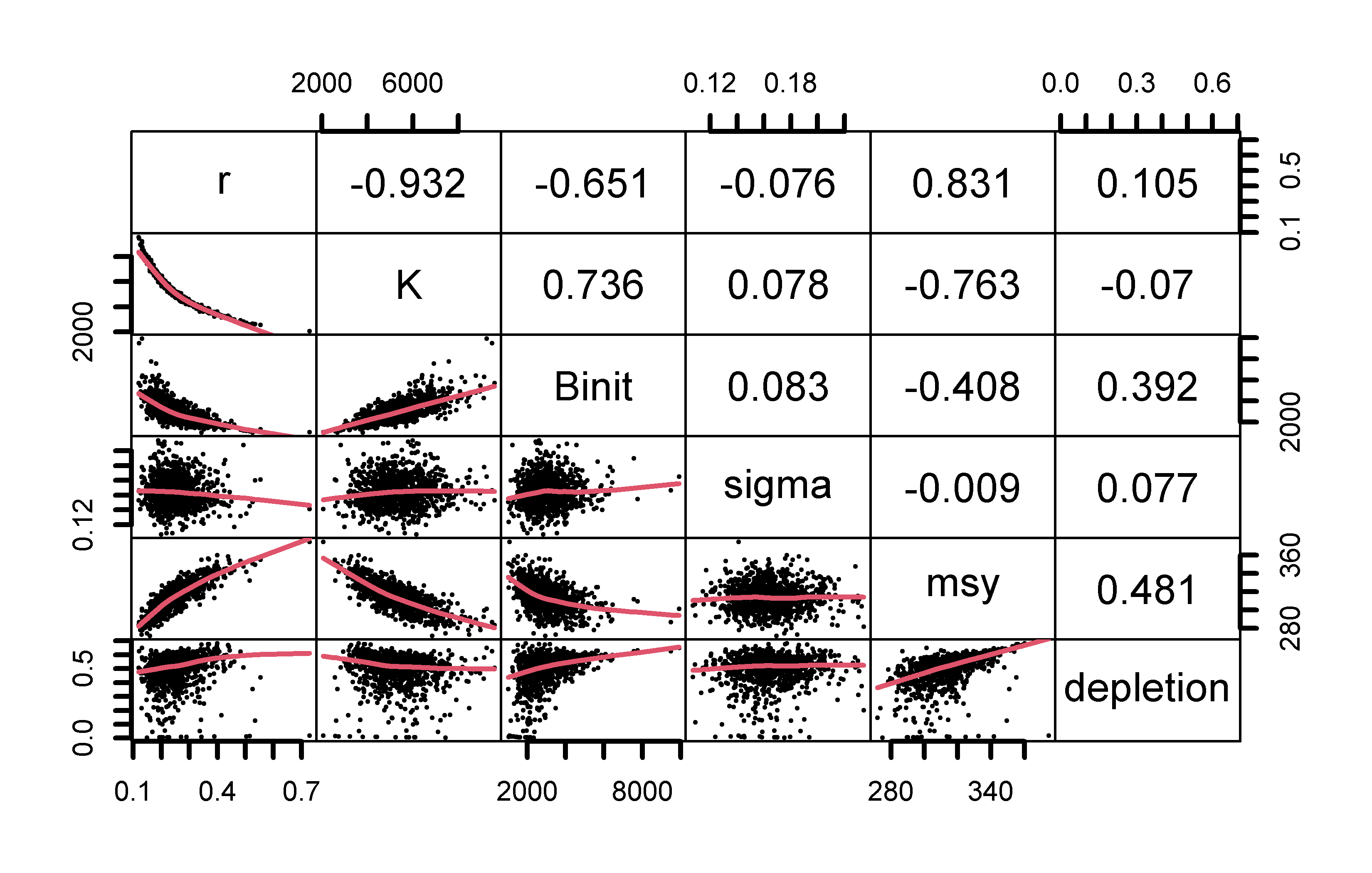
Figure 7.19: The relationships between the model parameters for the Schaefer model when using the multi-variate normal distribution to generate the parameter combinations. The relationship between r - K is much tighter than in the bootstrap samples and there is almost no relationship between sigma and the other parameters. The depletion plots indicate some trajectories go extinct.
We can compare the ranges of the parameter values from the bootstrap sampling and the asymptotic error sampling. The parameter samples from the asymptotic errors distribution are less skewed than from the bootstrap, but the bootstrap does not have such low values for \(B_{init}\) and \(K\). It needs to be remembered that the use of the multi-variate Normal distribution to describe the shape of the likelihood surface around the optimum parameter set remains only an approximation.
 # Get the ranges of parameters from bootstrap and asymptotic
bt <- apply(bootpar,2,range)[,c(1:4,6,7)]
ay <- apply(mvnpar,2,range)
out <- rbind(bt,ay)
rownames(out) <- c("MinBoot","MaxBoot","MinAsym","MaxAsym") | r | K | Binit | sigma | MSY | Depl | |
|---|---|---|---|---|---|---|
| MinBoot | 0.0653 | 3139.827 | 1357.264 | 0.1125 | 217.164 | 0.0953 |
| MaxBoot | 0.4958 | 25666.568 | 8000.087 | 0.1636 | 530.652 | 0.7699 |
| MinAsym | 0.1185 | 2055.714 | 1003.558 | 0.1069 | 271.901 | 0.0054 |
| MaxAsym | 0.7287 | 9581.273 | 9917.274 | 0.2344 | 374.522 | 0.6820 |
7.4.5 Sometimes Asymptotic Errors Work
In some cases the asymptotic errors approach generates results remarkably similar to those from the bootstrap. If we had used the abdat data instead of dataspm we would have obtained results that appear indistinguishable from the same analysis conducted using bootstraps (see the bootstrap section in the chapter On Uncertainty for a comparison). The trajectories generated look very similar, Figure(7.20), and the pairwise plots are almost indistinguishable. As in the On Uncertainty bootstrap example, we have used rgb() colouring to ease the comparison, Figure(7.21).
 #repeat asymptotice errors using abdat data-set Figure 7.20
data(abdat)
fish <- as.matrix(abdat)
pars <- log(c(r=0.4,K=9400,Binit=3400,sigma=0.05))
ansA <- fitSPM(pars,fish,schaefer=TRUE,maxiter=1000,hess=TRUE)
vcovA <- solve(ansA$hessian) # calculate var-covar matrix
mvn <- length(fish[,"year"])
N <- 1000   # replicates
mvncpueA <- matrix(0,nrow=N,ncol=mvn,dimnames=list(1:N,fish[,"year"]))
columns <- c("r","K","Binit","sigma")
optparA <- ansA$estimate  # Fill matrix of parameter vectors
mvnparA <- matrix(exp(rmvnorm(N,mean=optparA,sigma=vcovA)),
                  nrow=N,ncol=4,dimnames=list(1:N,columns))
msy <- mvnparA[,"r"]*mvnparA[,"K"]/4
for (i in 1:N) mvncpueA[i,]<-exp(simpspm(log(mvnparA[i,]),fish))
mvnparA <- cbind(mvnparA,msy)
plot1(fish[,"year"],fish[,"cpue"],type="p",xlab="Year",ylab="CPUE",
      maxy=2.5)
for (i in 1:N) lines(fish[,"year"],mvncpueA[i,],col=8,lwd=1)
points(fish[,"year"],fish[,"cpue"],pch=16,cex=1.0) #orig data
lines(fish[,"year"],exp(simpspm(optparA,fish)),lwd=2,col=0) 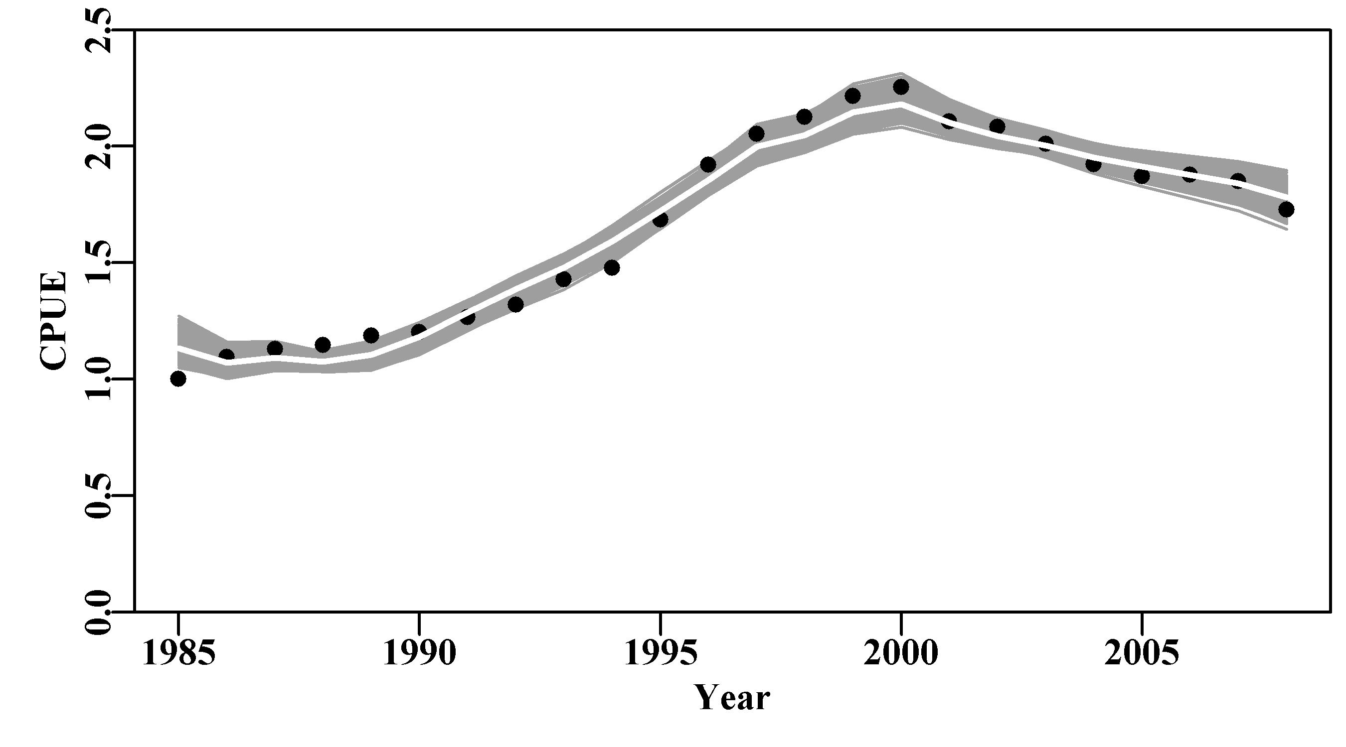
Figure 7.20: The use of asymptotic errors to generate plausible parameter sets and their implied cpue trajectories for the abdat data-set. The optimum model fit is shown as a white line.
 #plot asymptotically sampled parameter vectors Figure 7.21
pairs(mvnparA,lower.panel=panel.smooth, upper.panel=panel.cor,
gap=0,pch=16,col=rgb(red=0,green=0,blue=0,alpha = 1/10)) 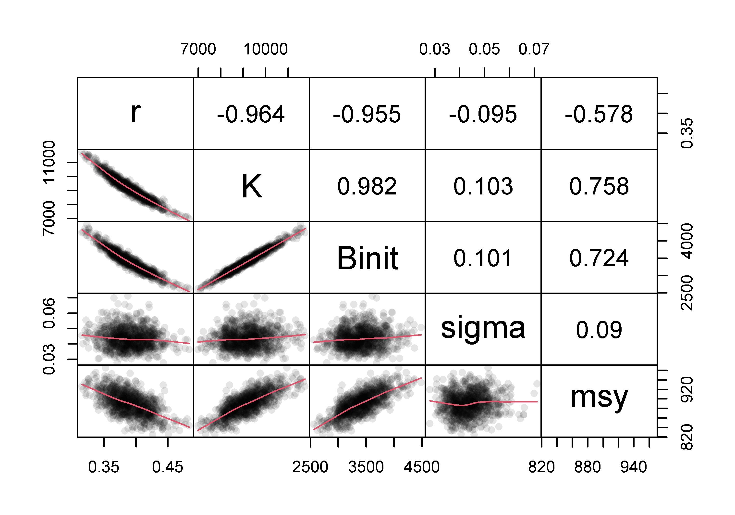
Figure 7.21: Model parameter relationships when fitting the Schaefer model to the abdat data and using the multi-variate normal distribution to generate subsequent parameter combinations. These are very similar to the bootstrap equivalent in the On Uncertainty chapter.
7.4.6 Bayesian Posteriors
We have already seen in the On Uncertainty chapter that it is possible to use a Markov Chain Monte Carlo (MCMC ) analysis to characterize the uncertainty inherent in a given analysis. Here we will use the abdat data-set again as that provides an example of very well behaved data leading to a relatively tightly fitting model and a well behaved MCMC analysis. The equations behind the Gibbs-within-Metropolis-Hastings (or single-component Metropolis-Hastings) strategy are given in the On Uncertainty chapter. These are all implemented in the do_MCMC() function. To use that it helps to first have an optimally fitting maximum likelihood based model. This time we will use the Fox model option.
 #Fit the Fox Model to the abdat data Figure 7.22
data(abdat); fish <- as.matrix(abdat)
param <- log(c(r=0.3,K=11500,Binit=3300,sigma=0.05))
foxmod <- nlm(f=negLL1,p=param,funk=simpspm,indat=fish,
              logobs=log(fish[,"cpue"]),iterlim=1000,schaefer=FALSE)
optpar <- exp(foxmod$estimate)
ans <- plotspmmod(inp=foxmod$estimate,indat=fish,schaefer=FALSE,
addrmse=TRUE, plotprod=TRUE) 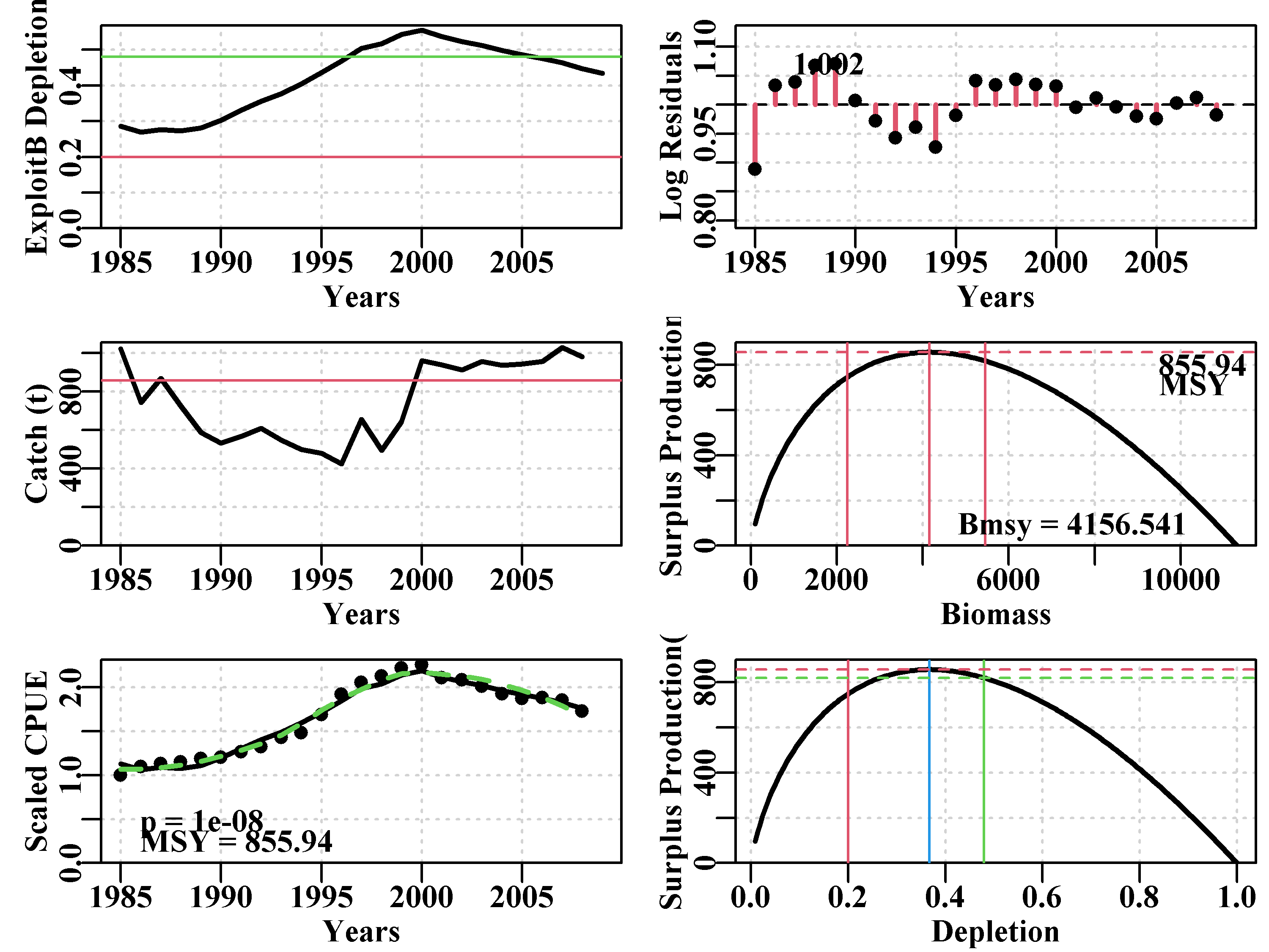
Figure 7.22: The optimum model fit for the abdat data-set using the Fox model and log-normal errors. The green dashed line is a smoother curve while the red line is the optimum predicted model fit. Note the pattern in the log-normal residuals indicating that the model has small inadequacies with regard to this data.
With the optimum, which will be somewhere near the posterior mode, we no longer have any need to illustrate the notion of a burn-in period but ideally we do not want to start from exactly the maximum likelihood solution. So we can round off the optimum solution and burn-in the Markov Chain so as to get the sequence of parameter sets to enter the bounds of plausible combinations. We know the \(r\) and \(K\) parameters are strongly correlated so we might use an initial step size of 128 (4 x 128 = 512) to try to reduce any auto-correlation between any sequentially accepted values, but this is also influenced by the relative scales applied to the jumps between parameter iterations. Here we started with values between one and two percent but experimented with those values until the acceptance rates lay between 0.2 and 0.4. It is best to do this with reduced N values (using a thinning of 512, even 1000 is half a million iterations). Only when the scales are appropriately set should one expand the replicates, N, out to some larger number to obtain clearer results. We will continue to use the MQMF function calcprior() to set equal weight on each set of plausible parameters, and to obtain repeatable results you would need to include a set.seed() call on each chain, but generally we would leave this out. The same random number generators are used in R for all operating systems so this should work across computers, but I haven’t tried this on all versions. To improve the speed of calculations it would be useful to have something akin to the simpspmC() function using Rcpp described in the On Uncertainty chapter. Before we run the following MCMC you will need to compile the appendix to this chapter or call simpspm() when using do_MCMC(), note the schaefer=FALSE argument is included in order to use the Fox model.
 # Conduct an MCMC using simpspmC on the abdat Fox SPM
 # This means you will need to compile simpspmC from appendix
set.seed(698381) #for repeatability, possibly only on Windows10
begin <- gettime()  # to enable the time taken to be calculated
inscale <- c(0.07,0.05,0.09,0.45) #note large value for sigma
pars <- log(c(r=0.205,K=11300,Binit=3200,sigma=0.044))
result <- do_MCMC(chains=1,burnin=50,N=2000,thinstep=512,
                  inpar=pars,infunk=negLL,calcpred=simpspmC,
                  obsdat=log(fish[,"cpue"]),calcdat=fish,
                  priorcalc=calcprior,scales=inscale,schaefer=FALSE)
 # alternatively, use simpspm, but that will take longer.
cat("acceptance rate = ",result$arate," \n")
cat("time = ",gettime() - begin,"\n")
post1 <- result[[1]][[1]]
p <- 1e-08
msy <- post1[,"r"]*post1[,"K"]/((p + 1)^((p+1)/p))
# acceptance rate = 0.3136629 0.3337832 0.3789844 0.3660627
# time = 15.58995The Fox model MCMC is currently setup with a thinning rate of 512, with 2000 replicates, and a burn-in of 50, meaning there will be 512 x 2050 = 1049600 iterations used to generate the required parameter traces. On the computer used to write this, even using simpspmC(), this took about 15 seconds; using simpspm() we might expect that to take about 75 seconds. Once this is known for your own system it is obviously possible to plan your analyses and make explicit choices over thinning rates and replicates (do not forget to use the latest version of R for the fastest times).
Once the analysis is complete we can plot each variable against the others using the pairs() function, Figure(7.23). But also we can plot the marginal posterior distributions for each main parameter and the derived model output (the MSY). Given we have used 2000 replicates with a chain thinning rate of 512, the posterior distributions are relatively smooth, Figure(7.24), although the few bumps present could be smoothed further by more replicates.
 #pairwise comparison for MCMC of Fox model on abdat  Fig 7.23
pairs(cbind(post1[,1:4],msy),upper.panel = panel.cor,lwd=2,cex=0.2,
lower.panel=panel.smooth,col=1,gap=0.1) 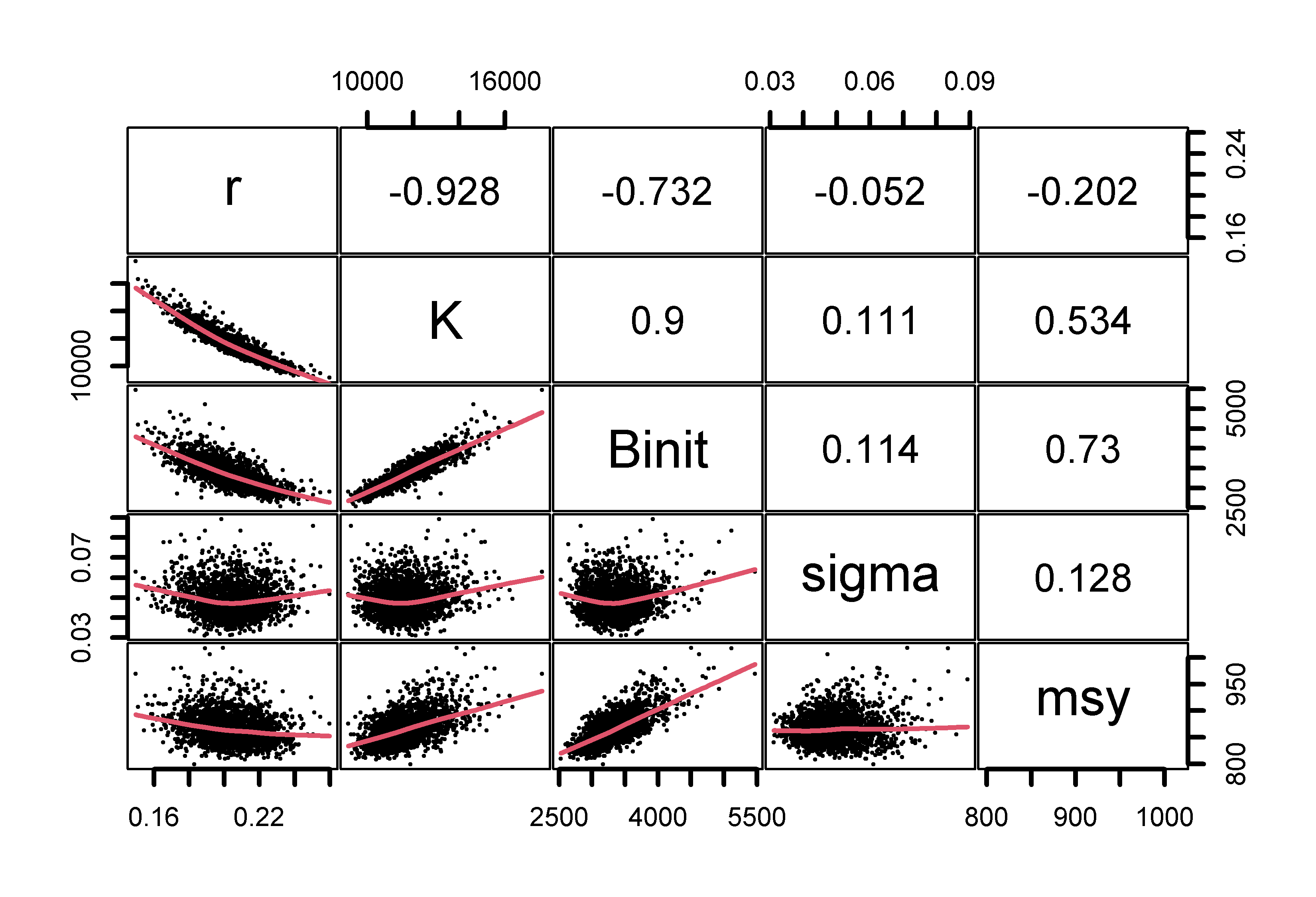
Figure 7.23: MCMC output as paired scattergrams. The solid lines are loess smoothers indicating trends and the numbers in the upper half are the correlation coefficients between the pairs. Strong correlations are indicated between r, K, and Binit, and between K, Binit, and MSY, with only minor or no relationships between sigma the other parameters or between msy and r.
 # marginal distributions of 3 parameters and msy  Figure 7.24
parset(plots=c(2,2), cex=0.85)
plot(density(post1[,"r"]),lwd=2,main="",xlab="r") #plot has a method
plot(density(post1[,"K"]),lwd=2,main="",xlab="K")   #for output from
plot(density(post1[,"Binit"]),lwd=2,main="",xlab="Binit")  # density
plot(density(msy),lwd=2,main="",xlab="MSY") #try str(density(msy)) 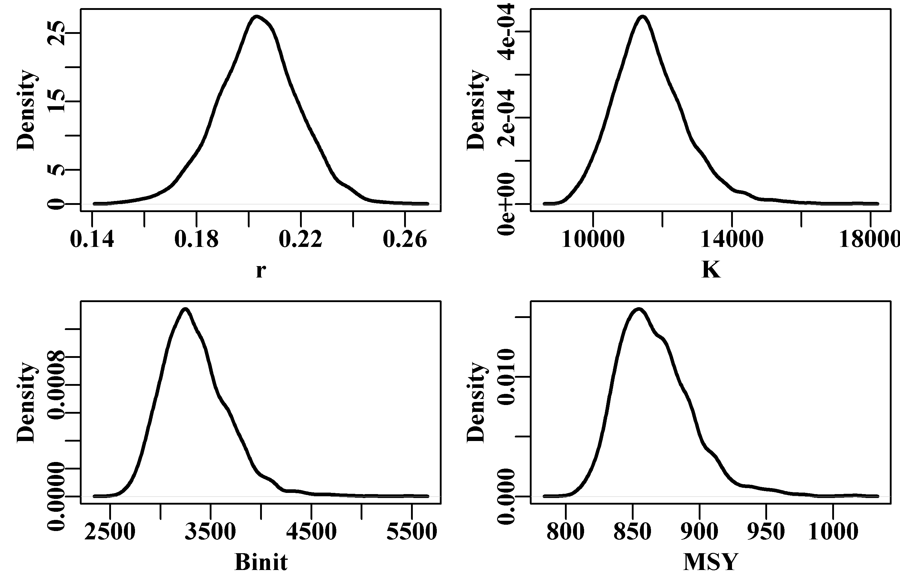
Figure 7.24: The marginal distributions for three parameters and the implied MSY from 2000 MCMC replicates for the Fox model applied to the abdat data. The lumpiness of the curves suggests more than 2000 iterations are needed.
Note that to get the acceptance rate for sigma down to less than 0.4 required a relatively large scaling factor to be imposed. The other parameters required values between 5 and 9 percent. If you used 500 replicates to search for the appropriate scaling factors and then reset the replicates to 2000, then the process will take four times as long. If you then increased the step size to say 1024 it would take double as long again. The search for appropriate scaling factors is needed to ensure the posterior space is well explored by the Markov Chain in a reasonable time. If the scaling were too small the acceptance rate would increase because each trial would effectively be very close to the original so only small steps could ever be taken. The stationary distribution will still be discovered eventually but it could take a very large number of replicates. With the thinning rate of 512, if you were to use the acf() function to plot the auto-correlation of any of the traces, as in acf(post1[,"r"]), you would find significant correlations still occur at steps of 1 and 2. To reduce those would require an increase to at least 1024.
As the number of replicates is increased the observed spread of potential parameter combinations increases. However, if we examine the bounds of the 90th percentile contours, these stay relatively stable. We can do this in two dimensions using the MQMF function addcontours(), which can generate contours for any arbitrary cloud of x-y data points (arbitrary but ideally smoothly distributed). The 50th and 90th percentile contours with 2000 observations is not particularly smooth, but even that has bounds for K approximately between about 9500 - 14000, and r between about 0.17 - 0.24, Figure(7.25). As the numbers increase the contours become smoother but their bounds remain approximately the same even though the x- and y-axes extend in both cases.
 #MCMC r and K parameters, approx 50 + 90% contours. Fig7.25
puttxt <- function(xs,xvar,ys,yvar,lvar,lab="",sigd=0) {
  text(xs*xvar[2],ys*yvar[2],makelabel(lab,lvar,sep="  ",
       sigdig=sigd),cex=1.2,font=7,pos=4)
} # end of puttxt - a quick utility function
kran <- range(post1[,"K"]);  rran <- range(post1[,"r"])
mran <- range(msy)         #ranges used in the plots
parset(plots=c(1,2),margin=c(0.35,0.35,0.05,0.1)) #plot r vs K
plot(post1[,"K"],post1[,"r"],type="p",cex=0.5,xlim=kran,
     ylim=rran,col="grey",xlab="K",ylab="r",panel.first=grid())
points(optpar[2],optpar[1],pch=16,col=1,cex=1.75) # center
addcontours(post1[,"K"],post1[,"r"],kran,rran,  #if fails make
            contval=c(0.5,0.9),lwd=2,col=1)   #contval smaller
puttxt(0.7,kran,0.97,rran,kran,"K= ",sigd=0)
puttxt(0.7,kran,0.94,rran,rran,"r= ",sigd=4)
plot(post1[,"K"],msy,type="p",cex=0.5,xlim=kran,  # K vs msy
     ylim=mran,col="grey",xlab="K",ylab="MSY",panel.first=grid())
points(optpar[2],getMSY(optpar,p),pch=16,col=1,cex=1.75)#center
addcontours(post1[,"K"],msy,kran,mran,contval=c(0.5,0.9),lwd=2,col=1)
puttxt(0.6,kran,0.99,mran,kran,"K= ",sigd=0)
puttxt(0.6,kran,0.97,mran,mran,"MSY= ",sigd=3) 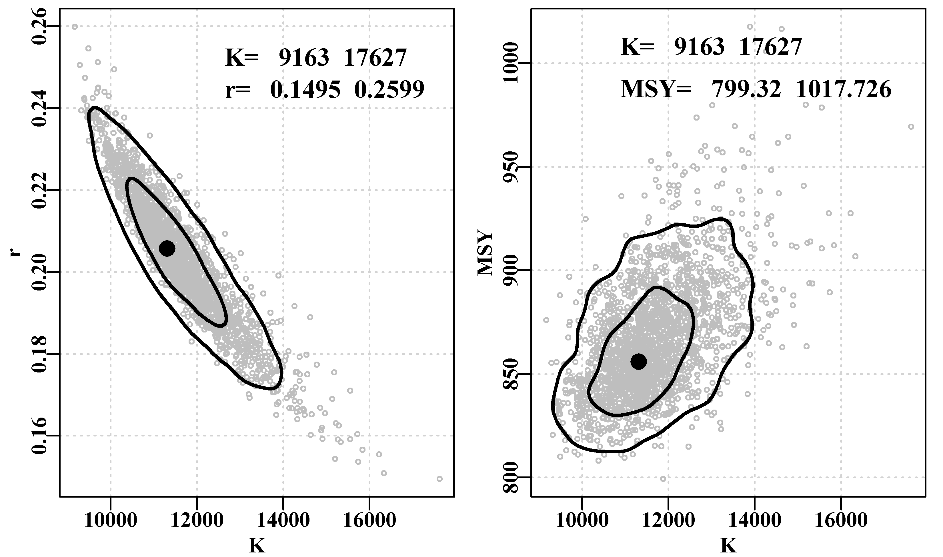
Figure 7.25: MCMC marginal distributions output as a scattergram of the r and K parameters, and the K and MSY values. The grey dots are from successful candidate parameter vectors, while the contours are approximate 50th and 90th percentiles. The text give the full range of the accepted parameter traces.
Finally, we can plot the individual traces for each of the 2000 replicates. This illustrates that even with the smooth marginal distributions occasionally there are spikes of parameter values that serve to illustrate the strong inverse correlation between the main parameters.
 #Traces for the Fox model parameters from the MCMC  Fig7.26
parset(plots=c(4,1),margin=c(0.3,0.45,0.05,0.05),
       outmargin = c(1,0,0,0),cex=0.85)
label <- colnames(post1)
N <- dim(post1)[1]
for (i in 1:3) {
  plot(1:N,post1[,i],type="l",lwd=1,ylab=label[i],xlab="")
  abline(h=median(post1[,i]),col=2)
}
msy <- post1[,1]*post1[,2]/4
plot(1:N,msy,type="l",lwd=1,ylab="MSY",xlab="")
abline(h=median(msy),col=2)
mtext("Step",side=1,outer=T,line=0.0,font=7,cex=1.1) 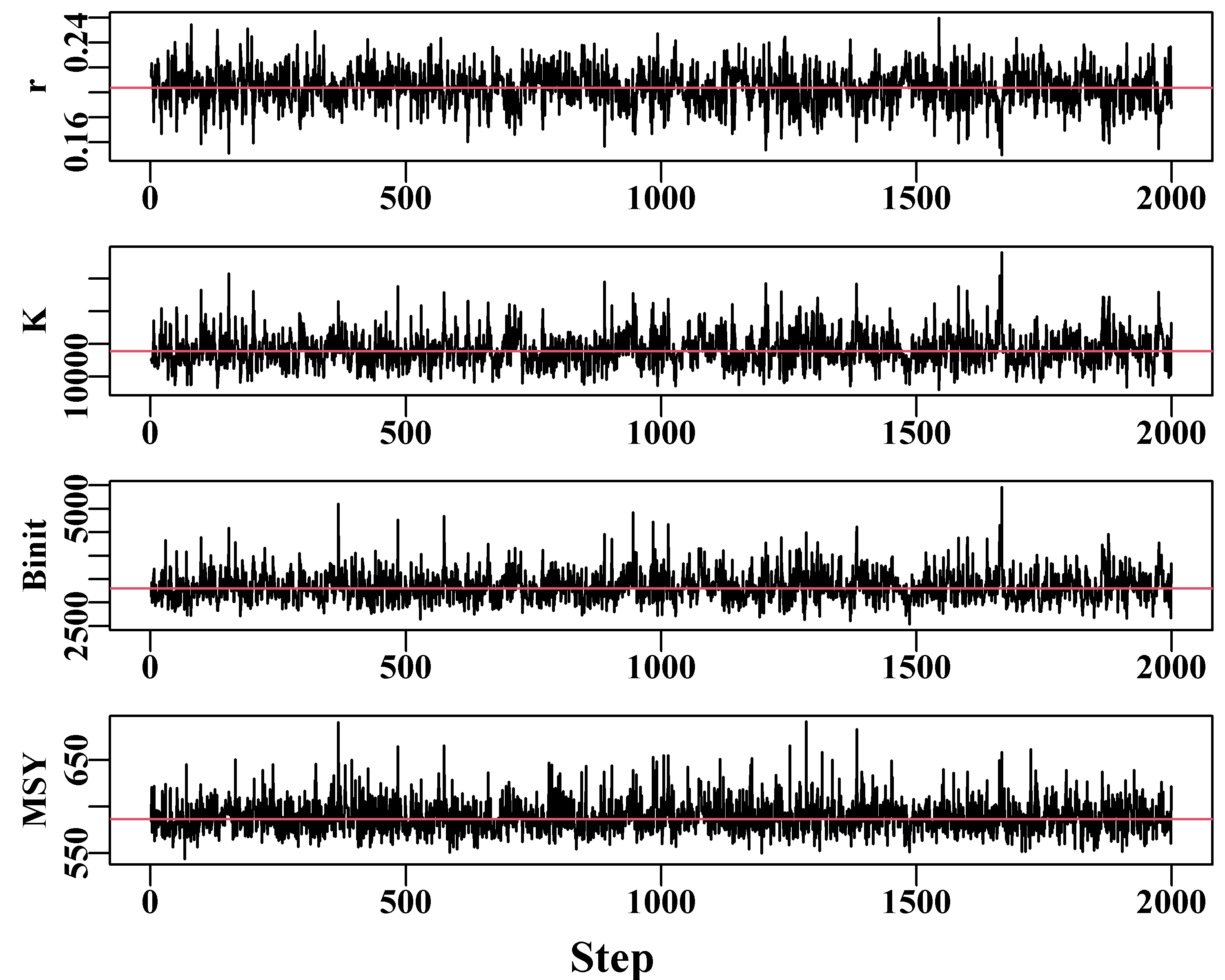
Figure 7.26: The traces for the three main Schaefer model parameters and the MSY estimates. The remaining auto-correlation within traces should be improved if the thinning step were increased to 1024 or longer.
Ideally, of course one would conduct such an analysis with multiple chains to ensure that they each converge of the same posterior distribution. In addition there are numerous diagnostic statistics to examine the rate of degree of convergence as the MCMC progresses. Equally ideally it would be best to start each chain from a different location, but the random number sequences eventually lead the chains in very different directions even if they start from the same place. One could use the same method of selecting different random starting points as was used in the robustSPM() function.
 #Do five chains of the same length for the Fox model
set.seed(6396679)  # Note all chains start from same place, which is
inscale <- c(0.07,0.05,0.09,0.45)  # suboptimal, but still the chains
pars <- log(c(r=0.205,K=11300,Binit=3220,sigma=0.044))  # differ
result <- do_MCMC(chains=5,burnin=50,N=2000,thinstep=512,
                  inpar=pars,infunk=negLL1,calcpred=simpspmC,
                  obsdat=log(fish[,"cpue"]),calcdat=fish,
                  priorcalc=calcprior,scales=inscale,
                  schaefer=FALSE)
cat("acceptance rate = ",result$arate," \n") # always check this
# acceptance rate = 0.3140023 0.3327271 0.3801893 0.36673 #Now plot marginal posteriors from 5 Fox model chains Fig7.27
parset(plots=c(2,1),cex=0.85,margin=c(0.4,0.4,0.05,0.05))
post <- result[[1]][[1]]
plot(density(post[,"K"]),lwd=2,col=1,main="",xlab="K",
ylim=c(0,4.4e-04),panel.first=grid())
for (i in 2:5) lines(density(result$result[[i]][,"K"]),lwd=2,col=i)
p <- 1e-08
post <- result$result[[1]]
msy <- post[,"r"]*post[,"K"]/((p + 1)^((p+1)/p))
plot(density(msy),lwd=2,col=1,main="",xlab="MSY",type="l",
ylim=c(0,0.0175),panel.first=grid())
for (i in 2:5) {
post <- result$result[[i]]
msy <- post[,"r"]*post[,"K"]/((p + 1)^((p+1)/p))
lines(density(msy),lwd=2,col=i)
} 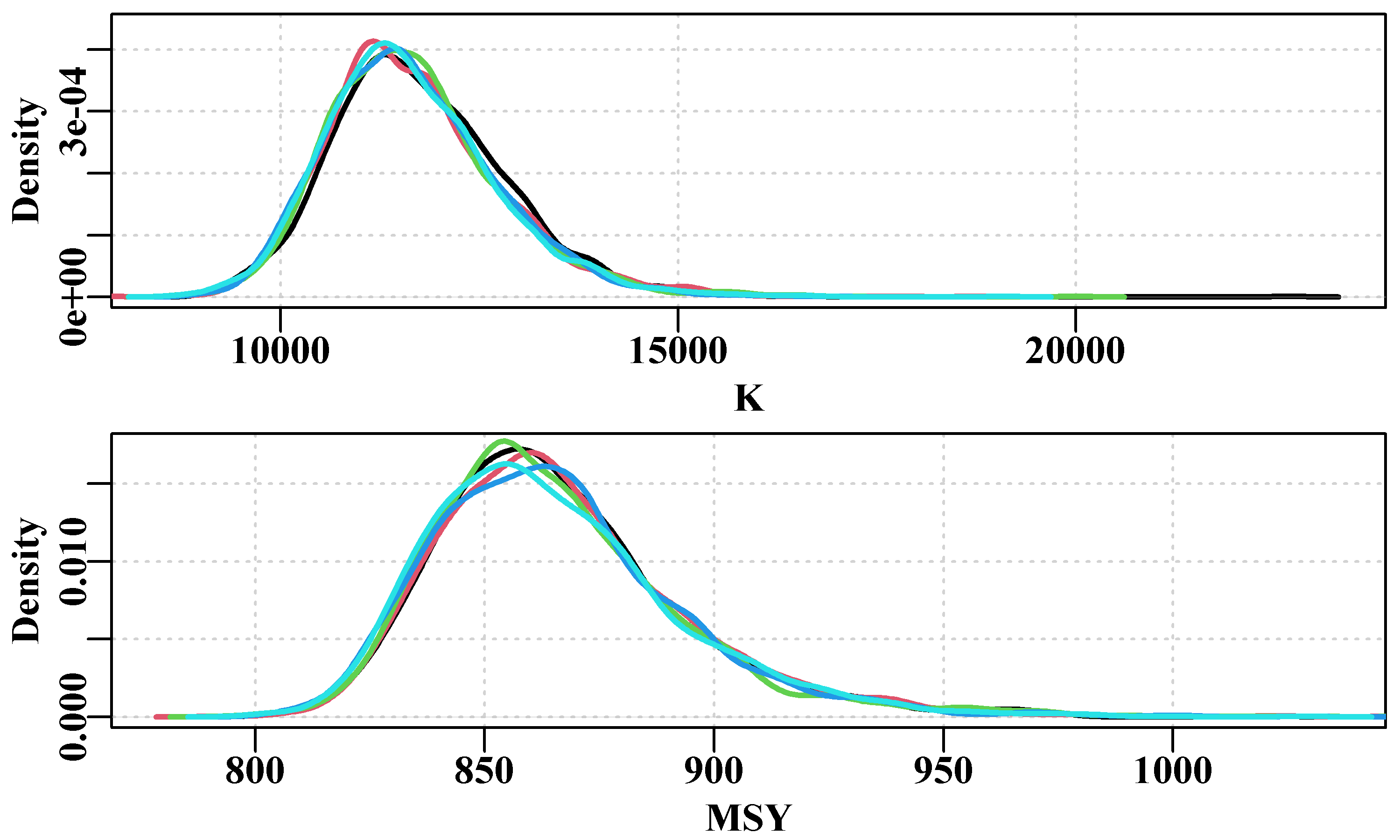
Figure 7.27: the marginal posterior for the K parameter and the implied MSY from five chains of 2000 replicates (512 * 2000 = 1049600 iterations). Some variation remains between the distributions, especially at the mode, suggesting that more replicates and potentially a higher thinning rate would improve the outcome.
However, despite the visual variation in the five chains, Figure(7.27), if we examine the \(K\) values at different quantiles we find few differences, Table(7.8). The fact that the median value of \(K\) for each chain are within about 1.1% of each other is encouraging and the maximum percent variation was on 2.7%. As an experiment, using the same random.seed, but running the chains each for 4000 steps, (a total of 5 x 512 * 4050 = 10.368 million iterations, but still less than five minutes), the maximum variation dropped to 1.48%, again for the 0.975 quantile, with the others all below 1%. In this case, with such a simple model and each chain only taking a short time, extending the number of steps is worthwhile. For more complex models with many more parameters and more complex calculation of the likelihood, the timing of these analyses can become critical when working to an assessment group deadline.
 # get qunatiles of each chain
probs <- c(0.025,0.05,0.5,0.95,0.975)
storeQ <- matrix(0,nrow=6,ncol=5,dimnames=list(1:6,probs))
for (i in 1:5) storeQ[i,] <- quants(result$result[[i]][,"K"])
x <- apply(storeQ[1:5,],2,range)
storeQ[6,] <- 100*(x[2,] - x[1,])/x[2,] | 0.025 | 0.05 | 0.5 | 0.95 | 0.975 |
|---|---|---|---|---|
| 9859.157 | 10160.471 | 11633.376 | 13740.430 | 14124.828 |
| 9893.256 | 10162.570 | 11541.118 | 13689.079 | 14302.523 |
| 9922.313 | 10157.503 | 11564.236 | 13620.369 | 14150.819 |
| 9875.521 | 10107.843 | 11541.843 | 13533.356 | 13908.780 |
| 9835.652 | 10088.899 | 11504.845 | 13640.376 | 14087.693 |
| 0.873 | 0.725 | 1.105 | 1.507 | 2.753 |
7.5 Management Advice
7.5.1 Two Views of Risk
A formal stock assessment, even a simple one using a surplus production model, gives one an indication of the stock status for the fishery being assessed but the question remains how is this used to generate fisheries management advice. Of course, such advice would depend upon what management objectives are in place for the fishery concerned. But even in the absence of a formal fishery policy it should be possible to provide advice on the implications of applying different levels of catch into the future. We can use the optimal model fit to project the model dynamics into the future and such projections are the foundation of the management advice that derives from most stock assessments that are not purely empirical. Once the objective for a fishery is known (or assumed) then, using model projections, it is possible to generate estimate of future effort or catch levels that would be expected to guide the stock to a selected objective.
A common objective is to try to maintain a fishery at a biomass level that can, on average, generate the maximum sustainable yield, this would be termed \(B_{MSY}\). Such an objective would be referred to as a target reference point as it derives from the literature that discussed biological reference points (Garcia, 1994; FAO, 1995, 1997). \(B_{MSY}\) may be considered a target but the associated catch (MSY) should really be coinsidered as an upper limit to catches. In addition to a target reference point there is usually a limit reference point, which defines a stock state to be avoided. This is often discussed in terms of stock levels perceived to pose a risk to subsequent recruitment, although this is generally only a guideline. Commonly, a limit reference point of \(B_{MSY}/2\) is used, or a common proxy for this is set at \(0.2B_0\). Such limit and target reference points are generally set in the context of a formal harvest strategy.
7.5.2 Harvest Strategies
Within a jurisdiction, a harvest strategy defines the decision framework to be used to achieve defined biological, and sometimes economic and social, objectives for different fish stocks. Generally a harvest strategy will have three components (FAO, 1995, 1997; Haddon, 2007; Smith et al, 2008):
a means of monitoring and collecting data with regard to each fishery of interest.
a defined manner in which each fishery is to be assessed, usually relative to pre-selected biological (or other) reference points such as fishing mortality rates, biomass levels, or their proxies.
pre-defined harvest control rules, or decision rules, that are used to translate a stock assessment or stock status into management advice relating to future effort or catch levels.
Ideally, such harvest strategies will have been simulation tested to determine the conditions under which they will be effective, and to reject options that fail to achieve the desired objectives (Smith, 1993; Punt et al, 2016)
There are a number of well known examples where management objectives for a jurisdiction’s fisheries have been stated explicitly (DAFF, 2007; Deroba and Bence, 2008; Magnuson-Stevens, 2007). In the Australian Commonwealth marine jurisdiction, for example, the target selected is to manage the primary economic stocks towards the biomass that generate the maximum economic yield, \(B_{MEY}\) (DAFF, 2007; DAWR, 2018); in fact a proxy of 0.48\(B_0\) is used for most species as insufficient information is available to reliably estimate \(B_{MEY}\). Similarly a proxy of 0.2\(B_0\) is defined as a limit reference point for the majority of species “Where information to support selection of a stock-specific limit reference point [\(B_{MSY}/2\)] is not available…” (DAWR, 2018, p 10). If a stock is estimated to be below the limit reference point then targeted fishing is stopped, although in mixed fisheries a bycatch can still occur. If a stock is above the limit reference point then projections are run to determine what future catches should encourage the stock to increase smoothly to target biomass levels.
7.6 Risk Assessment Projections
Of course, there are a number of important assumptions behind the idea of projecting a stock assessment model forwards. The first is that the model is successful in capturing the important parts of the dynamics controlling the stock biomass. With surplus production models this equates to assuming that the estimate of stock productivity will remain the same into the future. Remember that when using the data-set dataspm the residuals retained a relatively large oscillatory pattern indicating that the model was missing something important in the dynamics. Despite such omissions, the model might still retain a sufficient estimate of the approximate average dynamics to allow for useful projections, but that then assumes whatever other factors were influencing the model fit will continue to operate in the manner they did in the past. If an assessment is highly uncertain then future projections will also be highly uncertain, which lowers their value in terms of how confident one can be in providing advice.
The simplest projections are made using the optimal parameter estimates and imposing constant catches or effort. We would require the current stock biomass and the catchability to use the catch equation to convert a specified effort level into a catch level:
\[\begin{equation} C_t=qE_tB_t \tag{7.20} \end{equation}\]
Then the standard dynamics equation with the optimum parameters can be used to project the biomass levels forward under the predicted catch level. If using a specified catch level then we only need use the equation for the dynamics (here we use the Polacheck et al (1993) version):
\[\begin{equation} B_{t+1}=B_t+\frac{r}{p}B_t \left(1-\left(\frac{B_t}{K}\right)^p \right)-C_t \tag{7.21} \end{equation}\]
7.6.1 Deterministic Projections
If we were to use the optimum model parameters then for each of a range of different forward projected catches we would expect to obtain a different biomass and cpue trajectory. To exemplify this we can once again use the abdat data-set (note that we have set the hessian option to TRUE as we will use this later on).
 #Prepare Fox model on abdat data for future projections Fig7.28
data(abdat); fish <- as.matrix(abdat)
param <- log(c(r=0.3,K=11500,Binit=3300,sigma=0.05))
bestmod <- nlm(f=negLL1,p=param,funk=simpspm,schaefer=FALSE,
               logobs=log(fish[,"cpue"]),indat=fish,hessian=TRUE)
optpar <- exp(bestmod$estimate)
ans <- plotspmmod(inp=bestmod$estimate,indat=fish,schaefer=FALSE,
target=0.4,addrmse=TRUE, plotprod=FALSE) 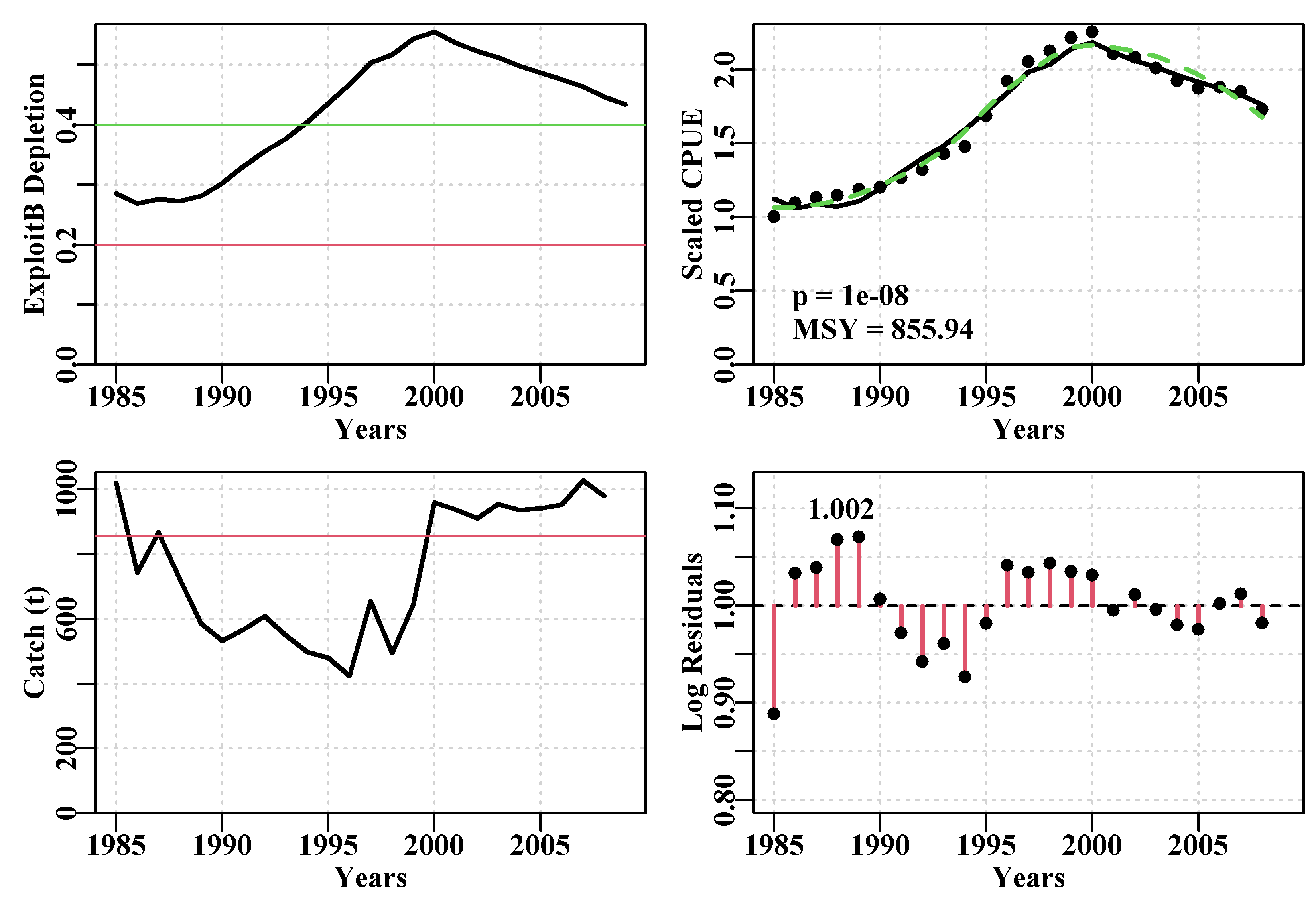
Figure 7.28: The optimum model fit for the abdat data-set using the Fox model and log-normal errors. The green dashed line is a loess curve while the solid red line is the optimum predicted model fit. Note the pattern in the log-normal residuals indicating that the model has some inadequacies with regard to this data.
The MSY estimate is about 854t and the stock appears to be just above a \(0.4B_0\) target level that often gets used as a proxy for \(B_{MSY}\). From the plot, and examining the original abdat data.frame, we can see that catches from 2000 to 2008 were between 910 - 1030t each year and that has led to the model predicting that the cpue and biomass would decline. We might thus explore a ten year projection of catches ranging from 700 - 1000t, perhaps in steps of 50t. Given the uncertainties in the analysis and that these projections are deterministic, there is little point in examining projections for too many years into the future. Long term projections can have value for illustrating the implications of different catches, but for practical purposes ten years would often be more than sufficient depending on the longevity of the species being assessed (longer lived species can be expected to exhibit slower dynamics than short lived species). The details of the dynamics that are plotted by the function plotspmmod() are generated by using the function spm() with the optimum parameters (look inside the code of plotspmmod() to see these details). The output of spm(), when run with the optimum parameters, includes the predicted dynamics in the outmat table within the Dynamics object. Here we will run the model using the Fox model rather than the Schaefer.
The object output by the function spm() is a list made up of five components. The model parameters, including the q value, the outmat is a matrix containing the dynamics through time, the msy, the sumout contains a summary of five key statistics, and schaefer identifies whether this is for a Schaefer or a Fox model.
# List of 5
#  $ parameters: Named num [1:5] 2.06e-01 1.13e+04 3.23e+03 4.38e..
#   ..- attr(*, "names")= chr [1:5] "r" "K" "Binit" "Sigma" ...
#  $ outmat    : num [1:25, 1:7] 1985 1986 1987 1988 1989 ...
#   ..- attr(*, "dimnames")=List of 2
#   .. ..$ : chr [1:25] "1985" "1986" "1987" "1988" ...
#   .. ..$ : chr [1:7] "Year" "ModelB" "Catch" "Depletion" ...
#  $ msy       : num 856
#  $ sumout    : Named num [1:5] 8.56e+02 1.00e-08 4.34e-01 2.86e..
#   ..- attr(*, "names")= chr [1:5] "msy" "p" "FinalDepl" "InitD"..
#  $ schaefer  : logi FALSE
The dynamics in outmat include details of the year, the biomass, the cpue, the predicted cpue, and other variables Table(7.9).
| Year | ModelB | Catch | Depletion | Harvest | CPUE | predCE | |
|---|---|---|---|---|---|---|---|
| 1985 | 1985 | 3231.104 | 1020 | 0.2856 | 0.3157 | 1.0000 | 1.1259 |
| 1986 | 1986 | 3043.856 | 743 | 0.2691 | 0.2441 | 1.0957 | 1.0607 |
| 1987 | 1987 | 3122.726 | 867 | 0.2761 | 0.2776 | 1.1303 | 1.0882 |
| 1988 | 1988 | 3082.459 | 724 | 0.2725 | 0.2349 | 1.1466 | 1.0741 |
| 1989 | 1989 | 3182.761 | 586 | 0.2814 | 0.1841 | 1.1873 | 1.1091 |
| 1990 | 1990 | 3426.923 | 532 | 0.3030 | 0.1552 | 1.2018 | 1.1942 |
| 1991 | 1991 | 3736.670 | 567 | 0.3303 | 0.1517 | 1.2652 | 1.3021 |
| 1992 | 1992 | 4020.992 | 609 | 0.3555 | 0.1515 | 1.3199 | 1.4012 |
| 1993 | 1993 | 4267.440 | 548 | 0.3773 | 0.1284 | 1.4284 | 1.4871 |
| 1994 | 1994 | 4575.104 | 498 | 0.4045 | 0.1088 | 1.4772 | 1.5943 |
A projection consists of taking a modelled time-series of results, such as in Table(7.9), and continuing the dynamics by sequentially including any new fixed catches and conducting the calculations to fill in the required columns. We can use the MQMF function spmprojDet(), which takes the list output from the spm() function along with some details relating to the deterministic projections, and generates the projected dynamics for us. You should examine the spmproj() code to see how the years are set up, the code is surprisingly brief.
 #  Fig 7.29
catches <- seq(700,1000,50)   # projyr=10 is the default
projans <- spmprojDet(spmobj=out,projcatch=catches,plotout=TRUE) 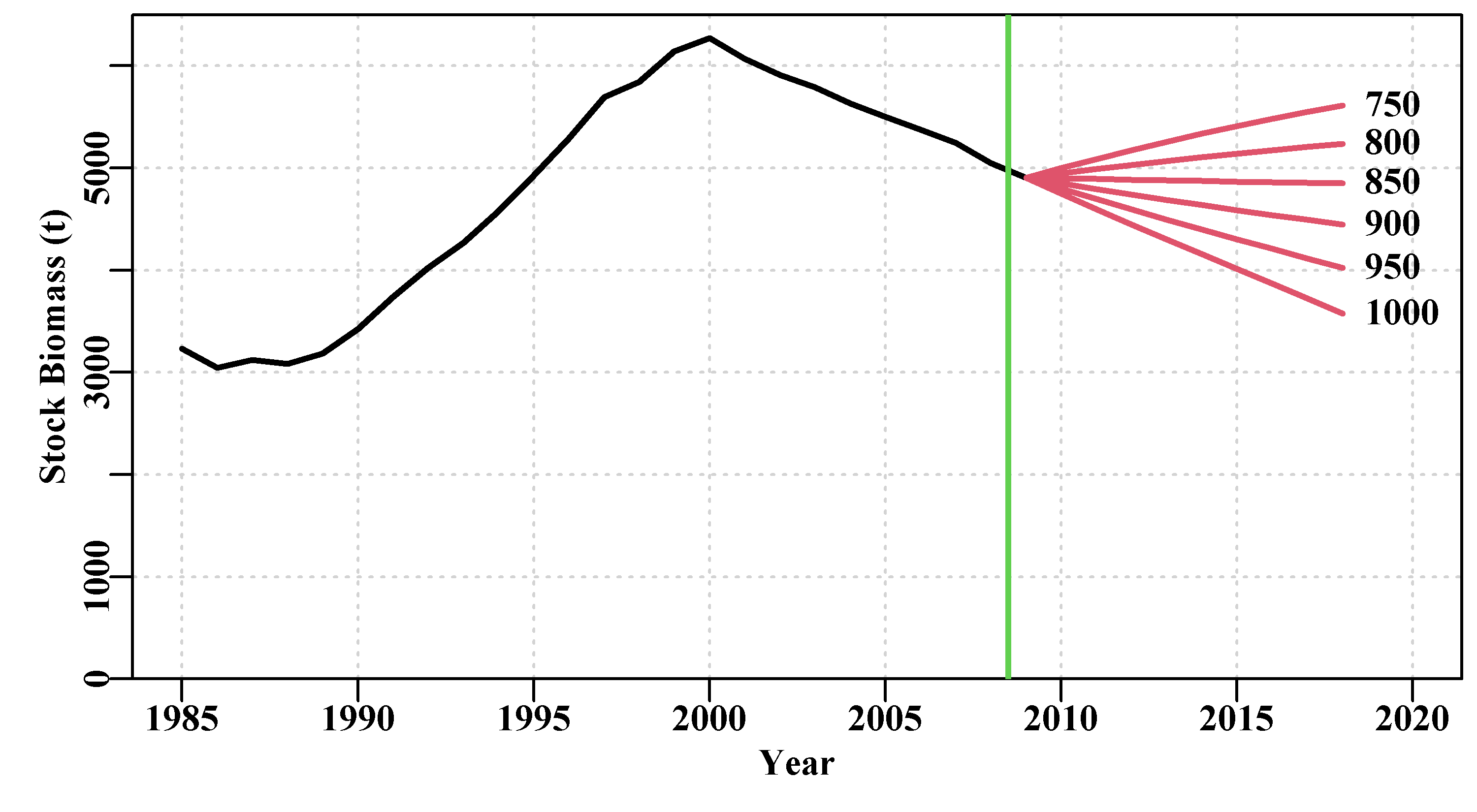
Figure 7.29: Deterministic constant catch projections of the optimum Fox model fit to the abdat data-set. the vertical green line is the limit of the data available and the red lines to the right of that are the main projections. The numbers are the constant catches imposed.
Using the deterministic constant catch projections, Figure(7.29), it can be seen that a constant catch of 850t, which is close to the MSY estimate, is the closest catch that predicts relatively stable stock conditions into the future.
7.6.2 Accounting for Uncertainty
An obvious problem with the deterministic projections is exactly the fact that they are deterministic. They fail to take any account of the uncertainty that remains even in the optimal model fit. Ideally we would conduct model projections while taking the estimated uncertainty into account. We can do this in three ways taking as a source of the uncertainty either the asymptotic errors approach, the bootstrap model fits, or the Bayesian approach. In each case, one output from the different analyses are lists of plausible parameter combinations. These can be used to describe the range of plausible dynamics included in the model fit and each of the separate biomass trajectories can be projected forward in the same manner as with the deterministic projections.
We have already calculated the hessian matrix when fitting the optimal model so we will start with an example where we use Asymptotic errors to generate a matrix of plausible parameter sets that we can then project forward.
7.6.3 Using Asymptotic Errors
Once we have an optimum model fit, if we have also calculated the hessian matrix, as we have seen, we can use the estimated asymptotic errors to generate a matrix full of plausible parameter vectors. These can then be used to generate replicate biomass trajectories which can then be plotted and summarized.
It is not uncommon to have probabilistic criteria for what constitutes successful fisheries management in terms of avoiding the limit reference point. With large numbers of replicate biomass trajectories, based upon different plausible parameter vectors, it is possible to estimate what proportion of projections will achieve a desired outcome. By tabulating the outcome of such projections managers can select the level of risk they deem appropriate. For example, an acceptable risk in the Australian Commonwealth Fishery Policy is explicitly defined such that “harvest strategies maintain the biomass of all commercial stocks above the Limit Reference Point at least 90% of the time.” And this is interpreted such that “the stock should stay above the limit biomass level at least 90% of the time (that is, a 1-in-10-year risk that stocks will fall below \(B_{LIM}\))” (DAWR, 2018a, p10).
In the section above we already have the optimum model fit for the abdat data-set using the Fox model surplus production (Polacheck et al, 1993). Just as we were able to generate the biomass trajectories when characterizing the uncertainty using the asymptotic errors, we can project each of those trajectories forward under a given constant catch and search for the catch level that produces the desired outcome. The first thing to do is to generate multiple plausible parameter vectors from the optimal model fit. We can use the function parasympt() to do this. Once the matrix of plausible parameter vectors is made we can then use spmproj() to project the dynamics forward for a given number of years and a given constant catch (once again check out its working by examining the code). parasympt() is merely a convenient wrapper for calling the rmvnorm() function (part of the package mvtnorm) and returning the result as a labelled matrix, spmproj() is slightly more complex. To simplify the projections, the function first extends the input fish matrix to include the projection years and their constant catches (filling in the future cpue with NA). The spmproj() uses the spm() function to calculate the dynamics, while only the modelled biomass is returned in a matrix. Using spm() may appear inefficient, but it means the spmproj() function can be easily modified to return any of the variables estimated in the dynamics. These variables include the model biomass, the depletion levels, the harvest rate, and the predicted cpue (though one can derive the rest from just the biomass, the predicted cpue, and the original data). Run the following code and examine the two output objects, matpar contains the parameter vectors, and projs contains the biomass trajectories as rows.
 # generate parameter vectors from a multivariate normal
 # project dynamics under a constant catch of 900t
library(mvtnorm)
matpar <- parasympt(bestmod,N=1000) #generate parameter vectors
projs <- spmproj(matpar,fish,projyr=10,constC=900)#do dynamics
Once calculated we can then summarize the results of the projections. First we can plot the 1000 projections using the function plotproj().
 # Fig 7.30  1000 replicate projections asymptotic errors
outp <- plotproj(projs,out,qprob=c(0.1,0.5),refpts=c(0.2,0.4)) 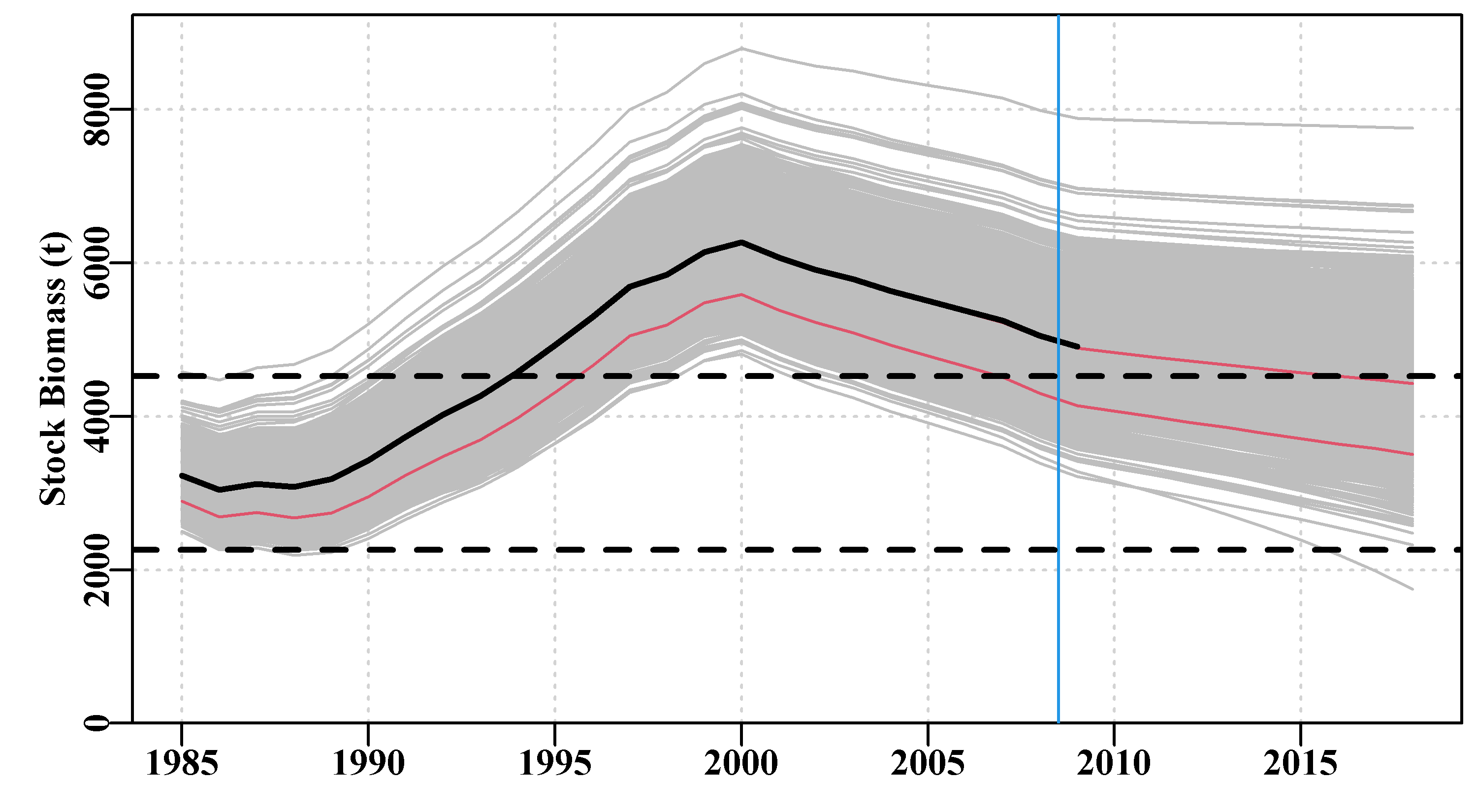
Figure 7.30: 1000 projections derived from the using the inverse hessian and mean parameter estimates to generate 1000 plausible parameter vectors and projecting each vector forward with the fisheries catches followed by 10 years of a constant catch of 900t. The dashed lines are the limit and target reference points. The blue vertical line is the limit of fisheries data, the thick black line is the optimum fit and the thin red lines parallel to the optimum line are the 10th and 50th quantiles across years.
It is clear that after 10 years, assuming the dynamics remain unchanged, catches of 900t, on average, leads the stock to decline somewhat from the present status but keeps the median outcome close to the target (upper dashed line) and the limit reference point (LRP) is not crossed by more than 10% of the trajectories after ten years (the lower thin line is above the \(0.2B_0\) limit. By exploring different constant catches you will be able to discover that if catches are increased to 1000t then after ten years the 10th quantile almost breaches the LRP. Tabulating what proportion of trajectories cross the LRP to generate a risk table would clarify the influence of different proposed constant catches and facilitates selection of more defensible management decisions.
7.6.4 Using Bootstrap Parameter Vectors
The essence of the projections is to generate a matrix of plausible parameter vectors from the optimum model fit combined with an estimation of the uncertainty inherent in the analysis. Instead of using the asymptotic errors with their assumed multi-variate normal distribution we can also use a bootstrapping process to generate the needed matrix of parameter vectors. Just as when we were characterizing the uncertainty in an analysis we can use the spmboot() function to create the required parameter vectors. If this function takes too long for comfort an alternative could be developed using the Rcpp based function simpspmC() to speed up the 1000 (or more) model fits.
 #bootstrap generation of plausible parameter vectors for Fox
reps <- 1000
boots <- spmboot(bestmod$estimate,fishery=fish,iter=reps,
                 schaefer=FALSE)
matparb <- boots$bootpar[,1:4] #examine using head(matparb,20)
Just as before we can use these parameter vectors to project the fishery forward and determine any risks to sustainability of different constant catch levels, Figure(7.31).
 #bootstrap projections. Lower case b for boostrap  Fig7.31
projb <- spmproj(matparb,fish,projyr=10,constC=900)
outb <- plotproj(projb,out,qprob=c(0.1,0.5),refpts=c(0.2,0.4)) 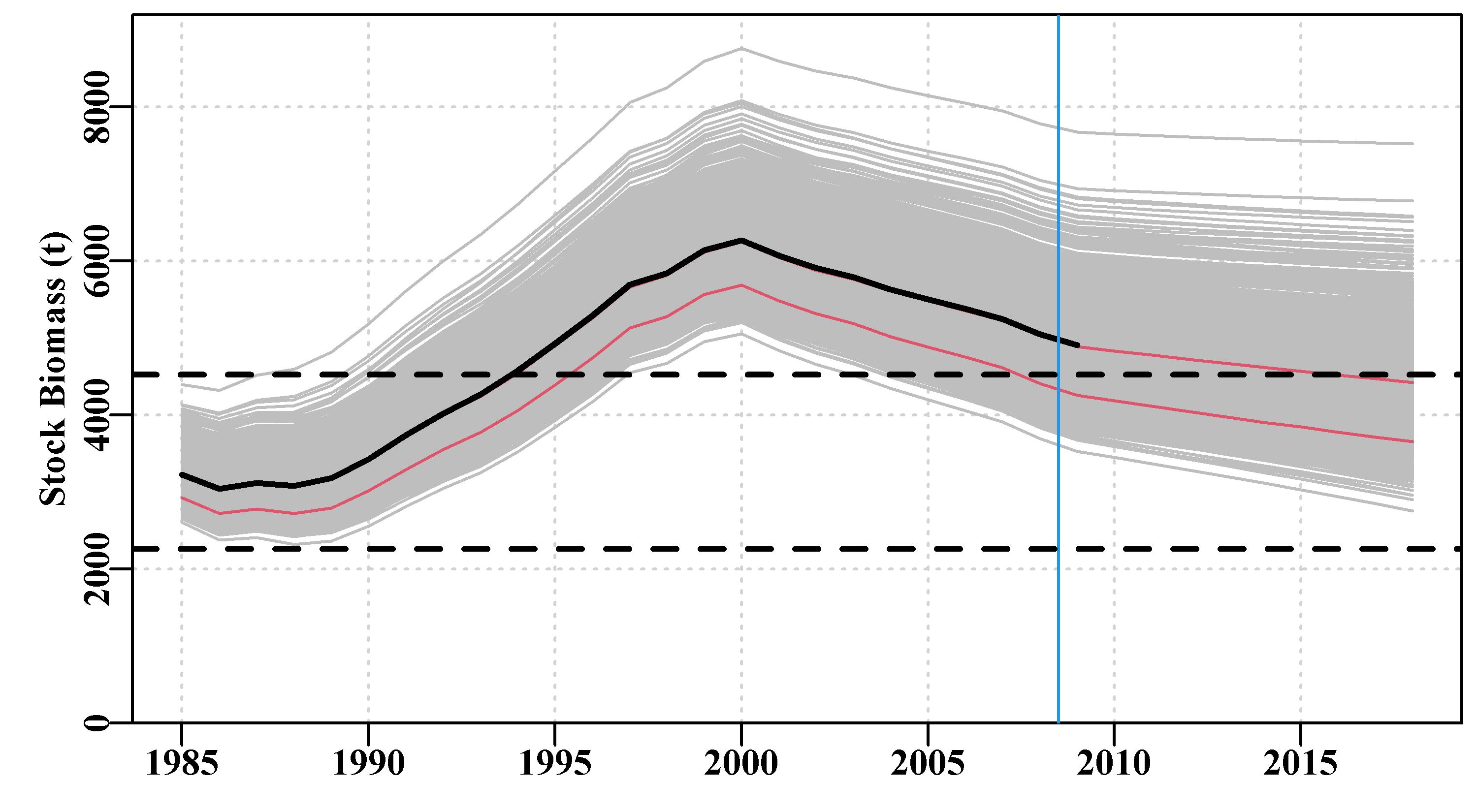
Figure 7.31: 1000 projections (in grey) derived from the using a bootstrap process to generate 1000 plausible parameter vectors and projecting each vector forward with the fisheries catches followed by 10 years of a constant catch of 900t. The dashed lines are the limit and target reference points. The blue vertical line is the limit of fisheries data, the thick black line is the optimum fit and the red lines are the 10th and 50th quantiles across years.
The projected grey lines differ (appear tighter around the median) from those generated using the asymptotic errors but the 10th and 50th quantiles look very similar. Certainly the summary outcome remains essentially the same, although, in this case, none of the projections fall below the Limit Reference Point (try outb$ltLRP and compare with outp$ltLRP).
7.6.5 Using Samples from a Bayesian Posterior
Just as we obtained samples from using asymptotic errors and bootstrap, it is possible to take samples from a Bayesian posterior to generate plausible parameter vectors. In this case we can use the function do_MCMC() to conduct the MCMC. We only need 1000 plausible parameter vectors so we will use a reasonable burn-in from a point close to the maximum likelihood maximum and use a large thinning rate to avoid serial correlation between sequential draws from the posterior distribution. As previously, it is best to use the Rcpp derived function simpspmC() to conduct the MCMC as we are still running with 2.145 million iterations. Because we are using the Fox implementation of the surplus production model the scaling factors are rather different from those used by the Schaefer version. If you have not compiled the simpspmC() function (listed in the appendix), then change the following code to use simpspm() and you can leave the as.matrix(fish) as it is to enhance speed.
 #Generate 1000 parameter vectors from Bayesian posterior
param <- log(c(r=0.3,K=11500,Binit=3300,sigma=0.05))
set.seed(444608)
N <- 1000
result <- do_MCMC(chains=1,burnin=100,N=N,thinstep=2048,
                  inpar=param,infunk=negLL,calcpred=simpspmC,
                  calcdat=fish,obsdat=log(fish[,"cpue"]),
                  priorcalc=calcprior,schaefer=FALSE,
                  scales=c(0.065,0.055,0.1,0.475))
parB <- result[[1]][[1]] #capital B for Bayesian
cat("Acceptance Rate = ",result[[2]],"\n")
# Acceptance Rate = 0.3341834 0.3087928 0.3504304 0.3506508To demonstrate that the resulting 1000 replicates have lost their serial correlation and represent a reasonable approximation to the stationary distribution we can plot the auto-correlation diagram and the trace of the 1000 replicate estimates of the \(K\) parameter, Figure(7.32).
 # auto-correlation, or lack of, and the K trace Fig 7.32
parset(plots=c(2,1),cex=0.85)
acf(parB[,2],lwd=2)
plot(1:N,parB[,2],type="l",ylab="K",ylim=c(8000,19000),xlab="") 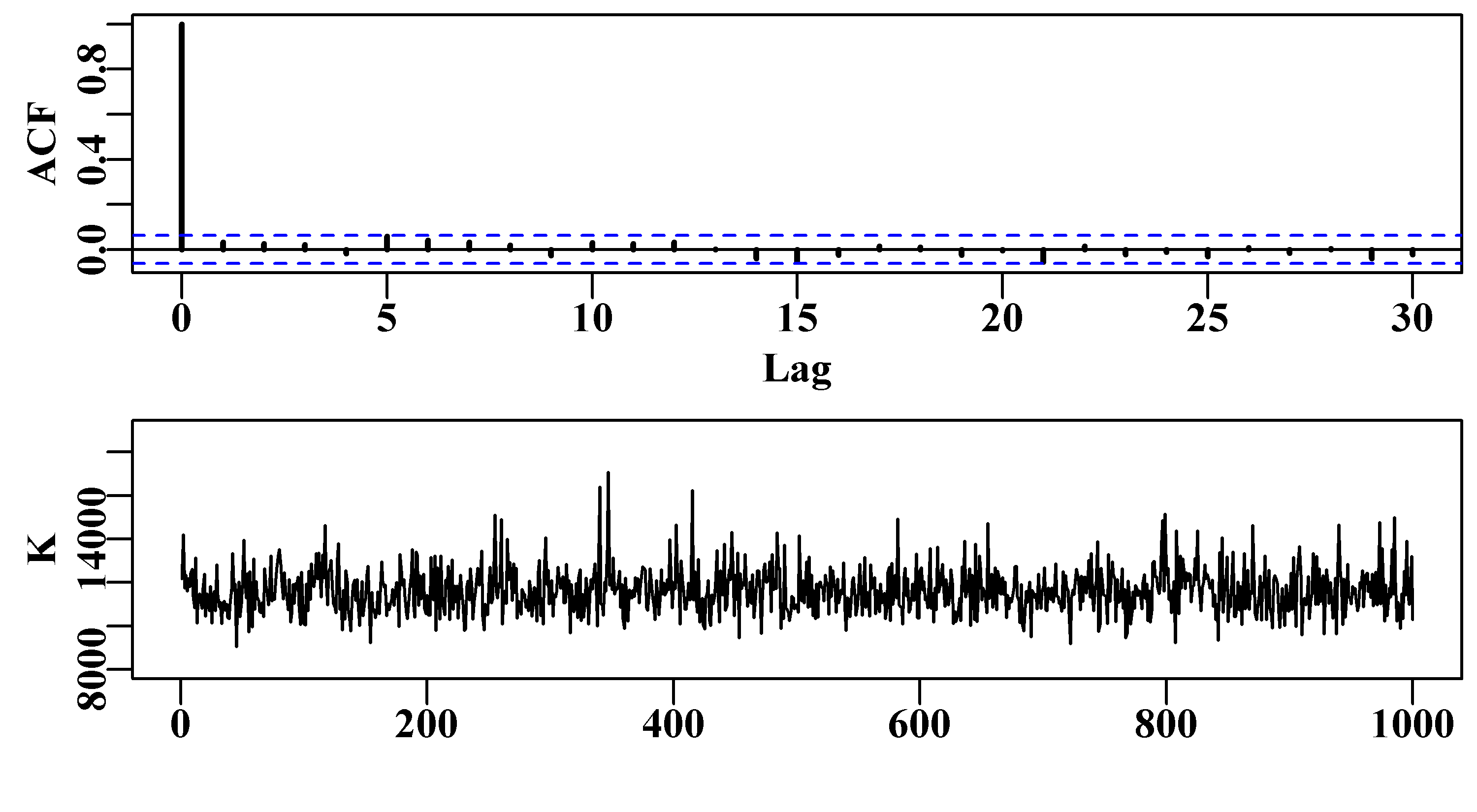
Figure 7.32: The lack of autocorrelation within 1000 draws from the posterior distribution for the K parameter for the Fox version of a surplus production model is apparent in the top plot. The trace in the bottom plot shows a typical scattering of values but retaining a few more extreme spikes.
These 1000 plausible parameter vectors can be extracted from the MCMC output and put through the same spmproj() and plotproj() functions as used previously, Figure(7.33).
 #  Fig 7.33
matparB <- as.matrix(parB[,1:4]) # B for Bayesian
projs <- spmproj(matparB,fish,constC=900,projyr=10) # project them
plotproj(projs,out,qprob=c(0.1,0.5),refpts=c(0.2,0.4)) #projections 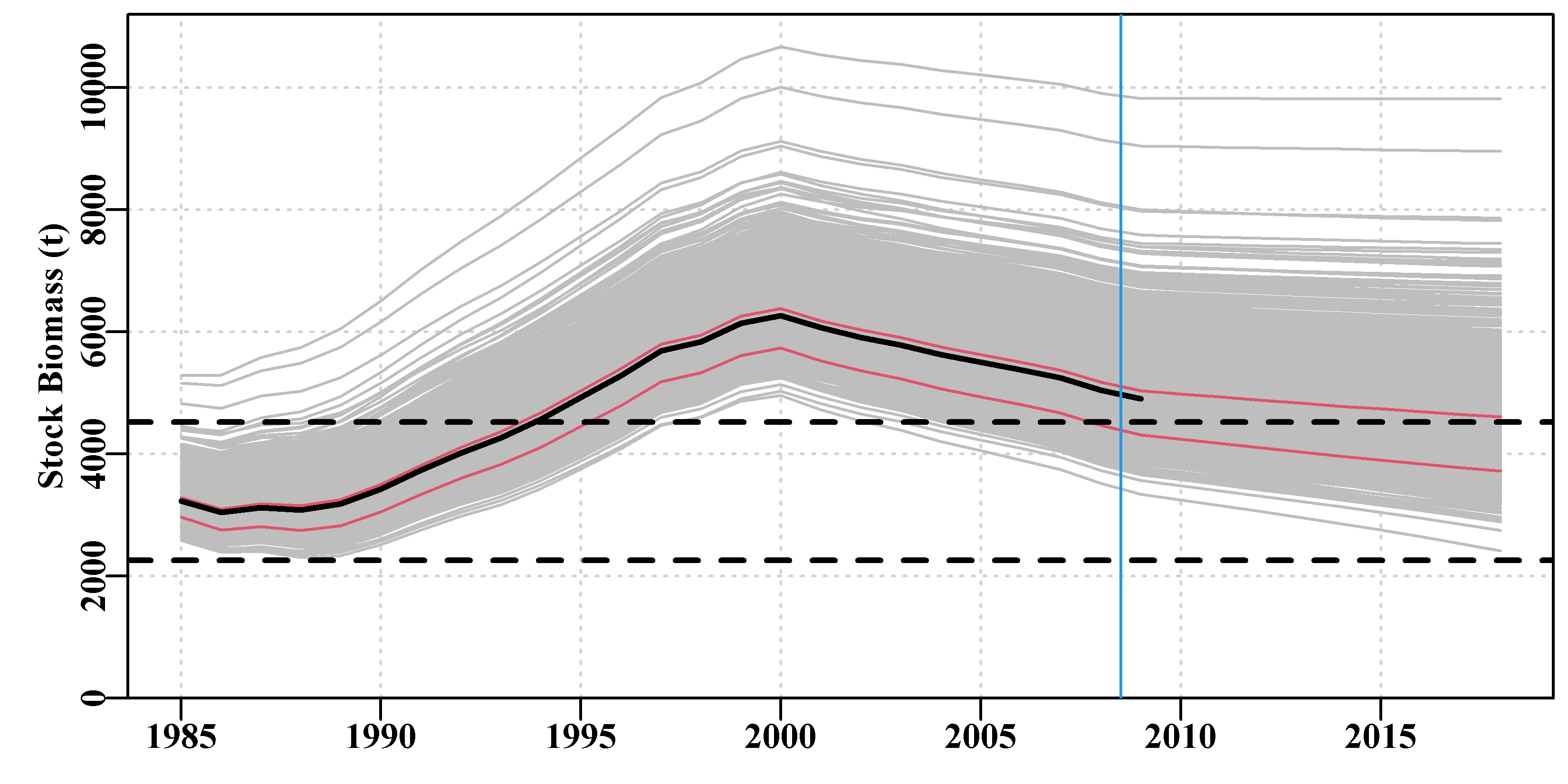
Figure 7.33: 1000 projections (in grey) of a constant catch of 900t, derived from the using 1000 samples from the Bayesian posterior. The dashed lines are the limit and target reference points. The blue vertical line is the limit of fisheries data, the thick black line is the optimum fit and the red lines are the 10th and 50th quantiles across years.
Note the median thin red line in Figure(7.33) (the 50th quantile) deviates slightly from the maximum likelihood optimum model fit line (black). But the 10th quantile remains in approximately the same place relative to the LRP as was observed in the analyses using the asymptotic errors and the bootstrap. Here there is a wider spread of biomass trajectories but the management outcomes would be very similar to the previous two approaches.
7.7 Concluding Remarks
We have examined in some detail how one might use a surplus production model to generate management advice for a fishery. The output might be a tabulation of the expected stock outcome under different catch or effort regimes for the next three to five years. Assuming that some management objective exists for the jurisdiction involved the managers can then make a decision and the fishery assessment scientists would be in a position to defend their results. Of course, given the uncertainty inherent in any fishery’s data and the vagaries of recruitment dynamics there can be no firm guarantees but with the assumptions that the stock dynamics will at least be similar to previous experience then a defense of the results is possible.
With the advent of climate change induced alterations to biological processes of growth and maturity we can also expect recruitment to be altered so clearly more care is needed. But large scale changes, if they occur due to a singular storm or other event, would constitute a new form of uncertainty that was unaccounted for in the assessment. This emphasizes the need to have assessment scientists who are aware of the what is happening in the regions within which the stocks live. No assessment, not even simple ones, should be made as merely an analytical, or mostly automated, exercise.
The reality is that the complexity and sophistication of an assessment is often associated with its relative value. The use of more complex models is only possible when there is an associated large increase in the available data for a fishery. There is thus a natural ordering of fish stocks with the most valuable usually receiving the most attention. However, all over the world, there is currently a large increase in interest, often driven by legal requirements, to provide management advice for even data-poor species. Thus, even though we have only reviewed relatively simple assessment methods these should not be spurned or neglected.
7.8 Appendix: The Use of Rcpp to Replace simpspm
In the Bayesian analysis, we wanted to use the Fox model of surplus production. This is certainly doable using the function simpspm() by altering the schaefer argument. However,
library(Rcpp)

cppFunction('NumericVector simpspmC(NumericVector pars,
             NumericMatrix indat, LogicalVector schaefer) {
   int nyrs = indat.nrow();
   NumericVector predce(nyrs);
   NumericVector biom(nyrs+1);
   double Bt, qval;
   double sumq = 0.0;
   double p = 0.00000001;
   if (schaefer(0) == TRUE) {
     p = 1.0;
   }
   NumericVector ep = exp(pars);
   biom[0] = ep[2];
   for (int i = 0; i < nyrs; i++) {
      Bt = biom[i];
      biom[(i+1)] = Bt + (ep[0]/p)*Bt*(1 - pow((Bt/ep[1]),p)) -
                          indat(i,1);
      if (biom[(i+1)] < 40.0) biom[(i+1)] = 40.0;
      sumq += log(indat(i,2)/biom[i]);
    }
    qval = exp(sumq/nyrs);
    for (int i = 0; i < nyrs; i++) {
      predce[i] = log(biom[i] * qval);
    }
    return predce;
}')