Chapter 5 Static Models
5.1 Introduction
In this book we are focussing on relatively simple population models but will also begin to prepare the way towards understanding some of the requirements of more complex models. By “more complex” we are referring to the age-structured models commonly used to model the dynamics of harvested populations. Nevertheless, we can use components of these more complex models to illustrate fitting of what we can call “static models” to data. Static models are used to describe the functional form of such processes as the growth of individuals, how maturity changes with age or size, the ‘stock-recruitment’ relationship between recruitment and mature or spawning biomass, and finally, the selectivity of fishing gear for a fished stock. Such static models exhibit a functional relationship between the variables of interest (length-at-age, maturity-at-age or -length, etc.) and these relationships are given the pretty big assumption of remaining fixed through time.
Such static models contrast with what we call dynamics models, which attempt to describe processes such as changes in population size, where the value being estimated at one time is a function of the population size at an earlier time. Such dynamics models invariably contain an element of self-reference, possibly along with other drivers, all of which contribute to the dynamics that we are attempting to describe or model.
In some situations, where clear changes have occurred in what are assumed to be static or stable processes, those would-be static relationships can be “time-blocked”, which implies that such relationships are assumed to change in a step-like fashion between two different time periods. In reality, changes to such processes, if they occur, are likely to have occurred more smoothly over a period of time, but unfortunately, having sufficient data to describe such gradual changes well is generally rare. With the advent of directionally changing sea temperatures and acidity through the effects of climate change, such alterations in processes such as growth and maturity can be expected to occur. But, as always, tracking any such changes will be data dependent. Generally, such processes are assumed to be constant or static, but as long as you are aware of the possibility of such changes this can be monitored and looked for.
We begin by implementing more examples with such models because, being static, as we saw in the Model Parameter Estimation chapter, they tend to be simpler to implement than models with sufficient flexibility to describe dynamic processes.
5.2 Productivity Parameters
By definition, all biological populations are made up of collections of individuals and, as such, exhibit emergent properties that partially summarize the properties of those populations. With the many extinctions currently under way I agree that just a few or even single individuals of a species might constitute some sort of limit to what constitutes a ‘population’, but we will focus only on more abundant populations and leave aside these sad extreme cases. Here we are going to focus on individual growth, maturity, and recruitment, all of which relate to a population’s productivity. A slow growing, late maturing, low fecundity species would tend to be less productive, though potentially more stable, than a fast growing, early maturing, highly fecund species. The evolution of life-history characteristics is a complex and fascinating subject, which I commend to your study (Beverton & Holt, 1959; Stearns, 1977, 1992). However, here we will focus on much simpler models. Even so, when modelling harvested populations a knowledge of the potential implications of the life-history characteristics of the species concerned should be very helpful in the interpretation of any observed dynamics. Do not forget that the modelling of biological processes benefits greatly from biological knowledge and understanding.
5.3 Growth
Ignoring any potential immigration and emigration, stock production is a combination of the recruitment of new individuals to a population and the growth of the individuals already in the population. Those are the positives, which are off-set by the negatives of natural mortality and, in harvested populations, fishing mortality. The importance of individual growth is one reason there is a huge literature on the growth of individuals in fisheries ecology (Summerfelt and Hall, 1987). Much of that literature relates to the biology of growth, which we are going to ignore, despite what I just wrote about the importance of understanding biological processes if you are going to model them. Instead, we will concentrate on the mathematical description of individual growth. The emphasis is on description, which is an important point because some people appear to get overly fond of particular growth models which only describe growth and do not really explain the process.
In the previous chapter on Model Parameter Estimation, we have already introduced three alternative models that can be used to describe length-at-age (von Bertalanffy, Gompertz, and Michaelis-Menton), so we will not re-visit those. Instead we will consider two other aspects of the description of growth. In terms of length-at-age, we will examine ideas relating to seasonal growth models, though these tend to be of limited use, though important in freshwater systems. More commonly used, we will also examine how one might estimate individual growth from tagging data.
In this chapter we will concentrate primarily on the von Bertalanffy growth curve and extensions to it using the function vB():
\[\begin{equation} L_t = L_{\infty} \left(1 - e^{-K(t - t_0)} \right ) \tag{5.1} \end{equation}\]
5.3.1 Seasonal Growth Curves
Growth rates can be complex processes affected by the length or age of each animal, but also by the environmental conditions. As a result, in temperate and polar regions, where the temperature can vary greatly through the year, growth rates can alter seasonally. This can be expressed as literal growth rings in the ear-bones (otoliths) of fish and other hard parts, that stem from changes in metabolism through the year. Of course, there are complications and obscurities brought about by other factors and events (for example, false rings in the hard parts), but again here we will focus on the description of the data assuming such complications have been dealt with before the analysis (reality often differs from this, do not under-estimate the difficulty of gathering valid fisheries data!).
Many different models of seasonal growth have been proposed but here we will use one proposed by Pitcher and Macdonald (1973), which modified the von Bertalanffy growth curve by including a sine wave into the growth rate term in an attempt to include cyclic water temperatures as a driver of growth rates such that they slowed in the winter and increased in the summer.
\[\begin{equation} {L}_{t}={{L}_{\infty }}\left( 1-{{e}^{-\left[ C\sin \left( \frac{2\pi \left( t-s \right)}{52} \right)+K(t-{{t}_{0}} \right]}} \right) \tag{5.2} \end{equation}\]
where \(L_{\infty}\), \(K\), and \(t_0\), are the usual von Bertalanffy parameters, \(t\) is the age in weeks at length \(L_t\), \(C\) determines the magnitude of the oscillations around the non-seasonal growth curve, \(s\) is the starting point in the year of the sine wave, and the use of the constant 52 reflects the use of weeks as the units of within-year time-step. If we had used months or days as the units of time measured between sampling events then we would have used 12 or 365 respectively. We can use the data that Pitcher and Macdonald (1973) produced on English freshwater minnows (Phoxinus phoxinus; though the minnow data were read from their plots, and is thus only approximately correct, but suffice for a demonstration).
We can begin by plotting the available data and fitting a standard non-seasonal von Bertalanffy growth curve. The curve is fitted using normal random errors rather than log-normal errors so we use the negNLL() function. It would be possible to use the ssq() function, but as we will be especially interested in the variation about the predicted curve we will stick with negNLL() in the following. If we ignore the seasonal trends then the expectation is that the variation around the curve (described by the sigma parameter), will be relatively large.
 #vB growth curve fit to Pitcher and Macdonald derived seasonal data
data(minnow); week <- minnow$week; length <- minnow$length
pars <- c(75,0.1,-10.0,3.5); label=c("Linf","K","t0","sigma")
bestvB <- nlm(f=negNLL,p=pars,funk=vB,ages=week,observed=length,
              typsize=magnitude(pars))
predL <- vB(bestvB$estimate,0:160)
outfit(bestvB,backtran = FALSE,title="Non-Seasonal vB",parnames=label)
# nlm solution: Non-Seasonal vB
# minimum : 150.6117
# iterations : 41
# code : 3 Either ~local min or steptol too small
# par gradient
# Linf 89.447640816 5.878836e-05
# K 0.009909338 2.705721e-01
# t0 -16.337065203 -4.717806e-05
# sigma 3.741419172 2.711341e-04The standard von Bertalanffy curve Equ(5.1), fitted to the seasonal data, has a sigma parameter of about 3.7, which merely reflects the fact that the data oscillate about the mean growth curve and so the residuals can be expected to be relatively large. The expectation is that if we used a seasonally adjusted curve this variation would be greatly reduced, we can therefore predict that sigma should be much smaller. To fit the seasonal growth curve we need to define a modified vB() function that reflects the new model structure, Equ(5.2). Of course, when fitting any new model the requirement of a function to generate predicted values from a set of parameters would invariably be the first step. It would be possible to include the calculation of the negative log-likelihood in that new function but keeping the generation of predicted lengths in a separate function increases the flexibility of our code. Hence, we will stick to the strategy of having separate functions for the prediction and the calculation of the negative log-likelihood. In the vector of parameters, pars, we will also need to include initial estimates of \(C\) and \(s\) from Equ(5.2).
 #plot the non-seasonal fit and its residuals.  Figure 5.1
parset(plots=c(2,1),margin=c(0.35,0.45,0.02,0.05))
plot1(week,length,type="p",cex=1.0,col=2,xlab="Weeks",pch=16,
      ylab="Length (mm)",defpar=FALSE)
lines(0:160,predL,lwd=2,col=1)
 # calculate and plot the residuals
resids <- length - vB(bestvB$estimate,week)
plot1(week,resids,type="l",col="darkgrey",cex=0.9,lwd=2,
    xlab="Weeks",lty=3,ylab="Normal Residuals",defpar=FALSE)
points(week,resids,pch=16,cex=1.1,col="red")
abline(h=0,col=1,lwd=1) 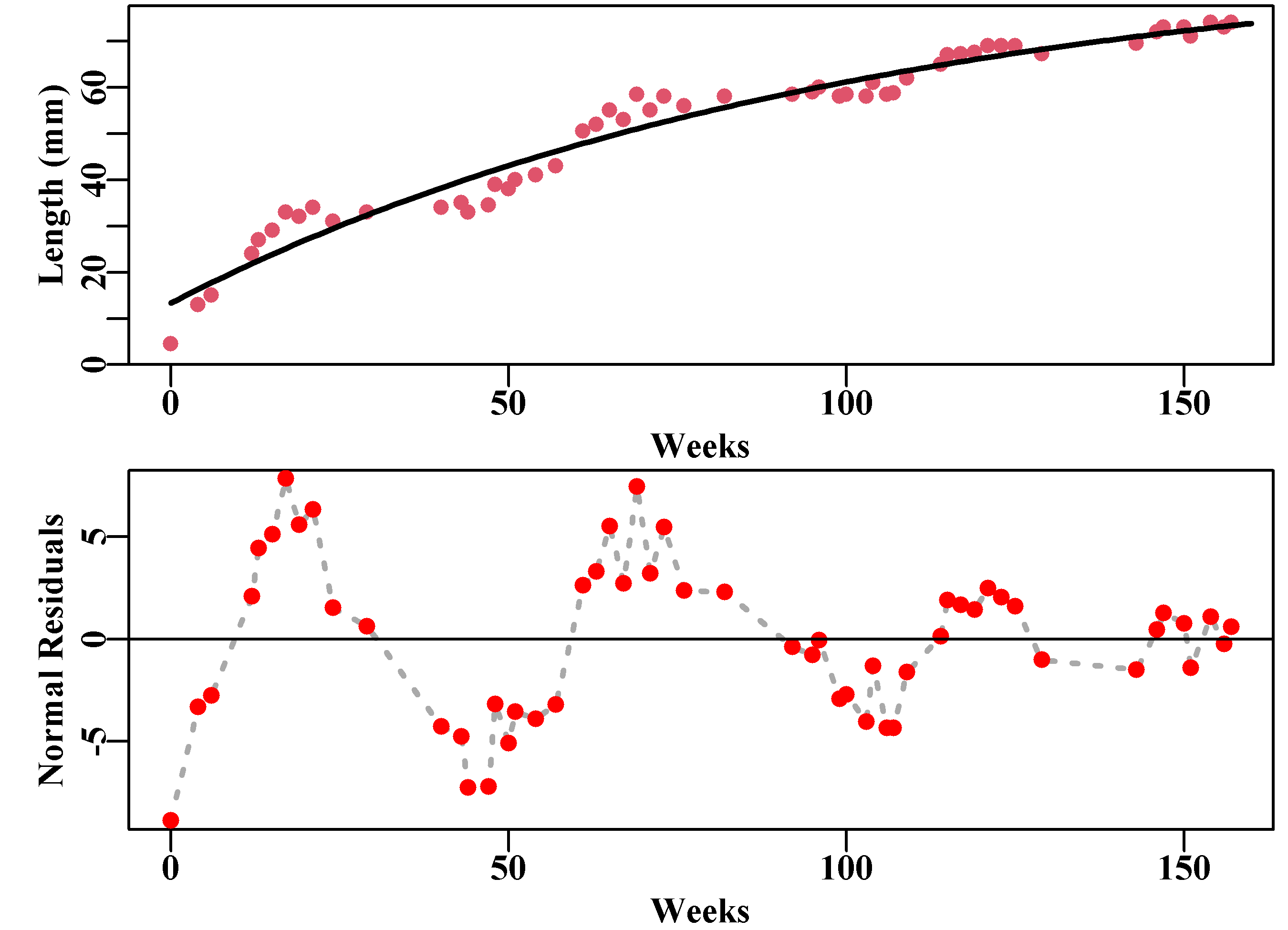
Figure 5.1: Length-at-age data derived from Pitcher and Macdonald (1973), illustrating strong seasonal growth fluctuations in growth rate when compared to the best fitting von Bertalanffy curve. The seasonal pattern in the normal random residuals in the bottom plot is very clear and reduces with age.
 # Fit seasonal vB curve, parameters = Linf, K, t0, C, s, sigma
svb <- function(p,ages,inc=52) {
  return(p[1]*(1 - exp(-(p[4] * sin(2*pi*(ages - p[5])/inc) +
                           p[2] * (ages - p[3])))))
} # end of svB
spars <- c(bestvB$estimate[1:3],0.1,5,2.0)  # keep sigma at end
bestsvb <- nlm(f=negNLL,p=spars,funk=svb,ages=week,observed=length,
              typsize=magnitude(spars))
predLs <- svb(bestsvb$estimate,0:160)
outfit(bestsvb,backtran = FALSE,title="Seasonal Growth",
       parnames=c("Linf","K","t0","C","s","sigma"))
# nlm solution: Seasonal Growth
# minimum : 105.2252
# iterations : 21
# code : 2 >1 iterates in tolerance, probably solution
# par gradient
# Linf 89.06448058 7.259952e-05
# K 0.01040808 3.973411e-01
# t0 -13.46176840 -5.575708e-05
# C 0.10816263 -5.358108e-03
# s 6.96964772 2.209217e-05
# sigma 1.63926525 7.775261e-05The seasonal adjustment to the growth rates only has minor effects on the \(L_{\infty}\) and \(K\) values, although it has a larger effect on the \(t_0\) value as the seasonality can allow for the initial rapid rise rather better than the standard vB() function. As expected the impact on the sigma parameter is great (3.74 down to 1.64). The improvement to the model fit is also large (-veLL down from 150 to 105 for the cost of adding two parameters). This is also reflected by a reduction in the pattern across the residuals and the halving of their maximum and minimum values as in Figure(5.2).
 #Plot seasonal growth curve and residuals   Figure 5.2
parset(plots=c(2,1))  # MQMF utility wrapper function
plot1(week,length,type="p",cex=0.9,col=2,xlab="Weeks",pch=16,
      ylab="Length (mm)",defpar=FALSE)
lines(0:160,predLs,lwd=2,col=1)
 # calculate and plot the residuals
resids <- length - svb(bestsvb$estimate,week)
plot1(week,resids,type="l",col="darkgrey",cex=0.9,xlab="Weeks",
      lty=3,ylab="Normal Residuals",defpar=FALSE)
points(week,resids,pch=16,cex=1.1,col="red")
abline(h=0,col=1,lwd=1) 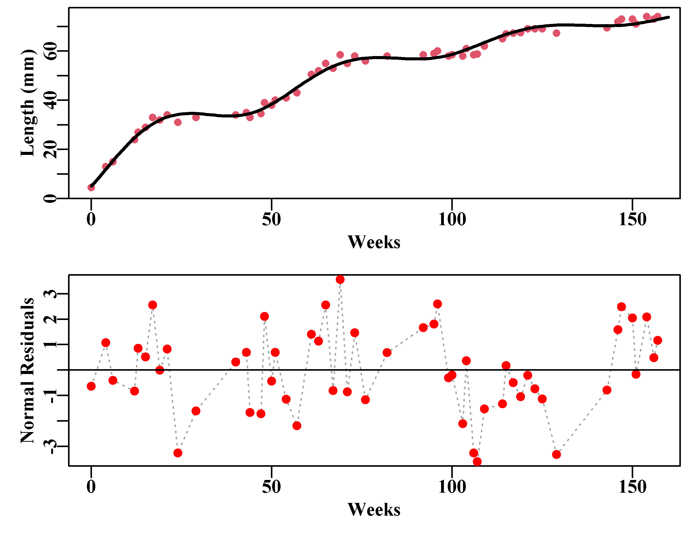
Figure 5.2: Approximate length-at-age data from Pitcher and Macdonald (1973) with a fitted seasonal version of the von Bertalanffy growth curve. The bottom plot is of the normal random residuals, which still have series of runs above and below zero but are less patterned than the non-seasonal curve.
This is certainly not the only growth curve available that allows for the description of seasonal variations in growth rate, but this section constitutes only an introduction to the principles. Indeed, there are very many alternative growth curves in the literature, with special cases for taxa such as Crustacea that grow in size through moulting. Thus, strictly, describing their growth involves estimating the growth increments from initial starting sizes and the duration and frequency of growth increments when they do moult. At a population level, however, if there are sufficient numbers, very often, a continuous growth curve can provide an adequate approximation of such growth within a population dynamics model.
Pitcher and Macdonald (1973) objected to the appearance of negative growth predicted by their first seasonal growth curve, but as they were dealing with samples of fish from a population and fitting to the mean of those samples, there is no biological reason why the mean of those samples could not decline slightly at times during the year. They also pointed out that using a direct fitting process “… took several hours on-line to a PDP 8-E computer with interactive graphics: however, an efficient optimization method would reduce this time considerably.” (Pitcher and Macdonald, 1973, p603). Hopefully, such a statement makes the reader more appreciate the now easy availability of non-linear optimizers and the remarkable computer speeds and the their analytical capacity (freely available software, like R, is truly empowering).
5.3.2 Fabens Method with Tagging Data
So far in the chapter on Model Parameter Estimation and here in Static Models, we have concentrated on length-at-age data, which obviously requires one to age the samples as well as measure their length. Unfortunately, not all animals can be aged with sufficient precision to enable such growth descriptions to be used. A common practice used from the very early days of fisheries related science is to tag and release fish (Petersen, 1896). Their recapture can be used to characterize movement and later, by measuring their length at tagging and at recapture it was used to describe the growth of the animals. Transformation of the equations used to describe more standard length-at-age curves is needed when using tagging data to fit the curves. Because we do not know the age of the tagged animals we need an equation that generates an expected length increment in terms of the von Bertalanffy parameters, the length at the time of tagging \(L_t\), and the length after the elapsed time, \(\Delta t\) would be \(L_{t+\Delta t}\). Fabens (1965) transformed the von Bertalanffy curve so it could be used with the sort of information obtained from tagging programs (see the Appendix to this chapter for the full derivation). By manipulating the usual von Bertalanffy curve Equ(5.1) Fabens produced the following:
\[\begin{equation} \begin{split} & \Delta \hat{L}={{L}_{t+\Delta t}}-{{L}_{t}} \\ & \Delta \hat{L}=\left( {{L}_{\infty }}-{{L}_{t}} \right)\left( 1-{{e}^{-K\Delta t}} \right) \end{split} \tag{5.3} \end{equation}\]
where, for an animal with an initial length of \(L_t\), \(\Delta L\) is the expected change in length through the duration of \(\Delta t\). By using the minimum least squares or negative log-likelihood one can estimate values for \(L_{\infty}\) and \(K\). To estimate a value for \(t_0\) one would require the average length-at-age for a known age so, generally, no \(t_0\) estimate can be made and the exact location of the growth curve along an age-axis is not determined. In such cases \(t_0\) is often set to zero.
If one can obtain data that records at least the initial size at tagging, the time interval between tagging and recapture, and the growth increment that occurs over that time interval, then we can put together a function to generate the required predicted growth increments given initial lengths and the two parameters \(L_{\infty}\) and \(K\), and then using maximum likelihood, we can obtain an optimum fit to whatever data we have.
This is best illustrated by plotting some tagging data, Figure(5.3, found in the MQMF data set blackisland for an abalone population). This includes a number of zero growth increments for some larger abalone. The data cloud is scattered (noisy) but some form of trend is apparent, and it is this trend that the growth models will attempt to fit.
 # tagging growth increment data from Black Island, Tasmania
data(blackisland);  bi <- blackisland # just to keep things brief
parset()
plot(bi$l1,bi$dl,type="p",pch=16,cex=1.0,col=2,ylim=c(-1,33),
     ylab="Growth Increment mm",xlab="Initial Length mm",
     panel.first = grid())
abline(h=0,col=1) 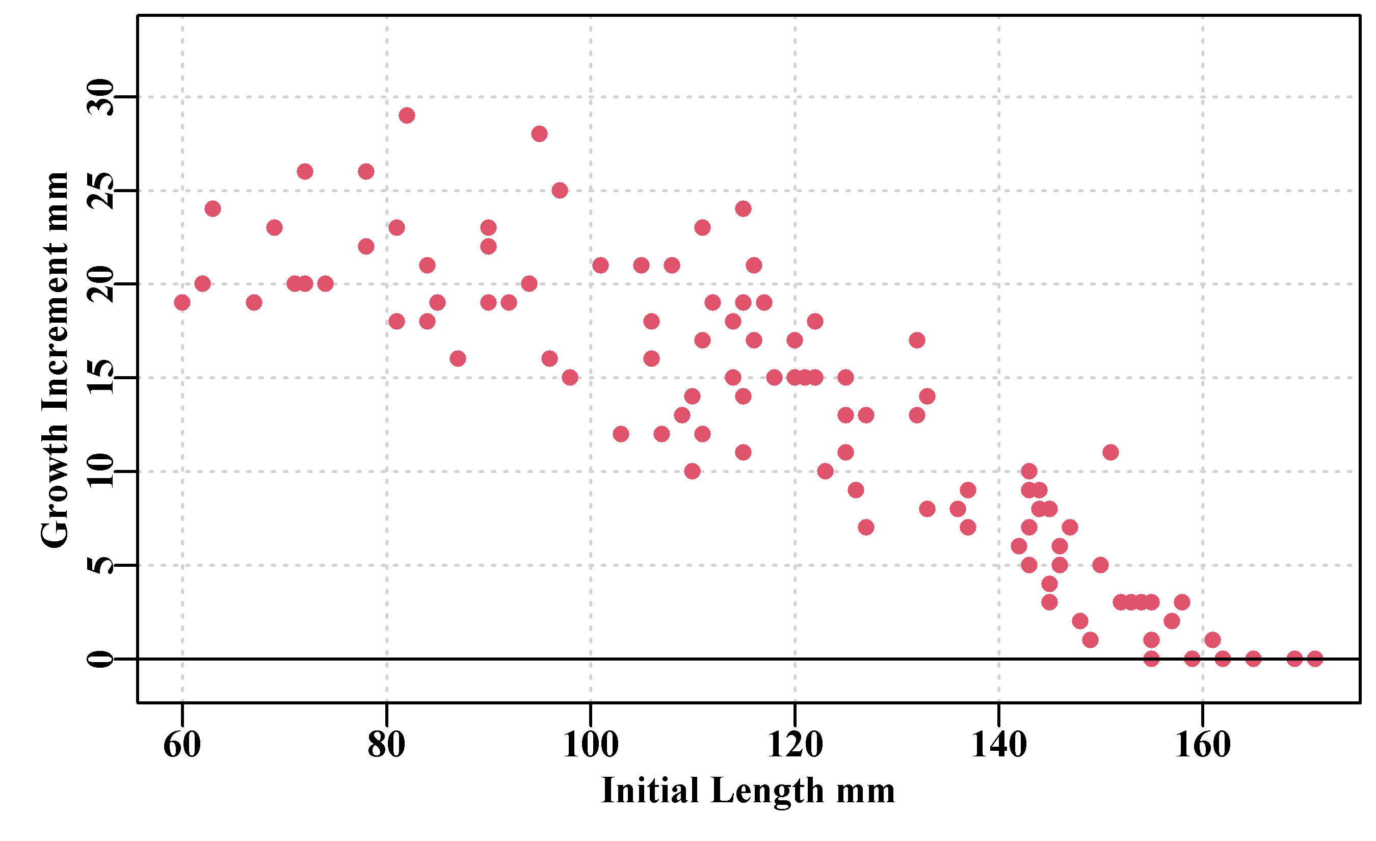
Figure 5.3: Tagging data collected for blacklip abalone from Black Island off the south-west corner of Tasmania. The time interval between tagging and recapture averaged 1.02 years.
As with the description of growth in the Model Parameter Estimation chapter, here we will fit and compare two growth curves to the example tagging data. These are the von Bertalanffy (Fabens, 1965; see Equ(5.3)), a standard for scalefish and many others species, and the inverse logistic (Haddon et al, 2008), which seems more suited to the indeterminate continuous growth exhibited by difficult to age invertebrates. The inverse logistic is more limited than the von Bertalanffy curve as it is designed to be used with time increments of one year, or at least a constant time increment
\[\begin{equation} \begin{split} \Delta L &= \frac{Max\Delta L}{1+{{e}^{log(19)({L_t}-L_{50})/\delta }}} + \varepsilon \\ {L_{t+1}} &= {L_t}+\Delta L + \varepsilon \end{split} \tag{5.4} \end{equation}\]
\(\delta\) is equivalent to \(L_{95} - L_{50}\), where \(L_{50}\) and \(L_{95}\) are the lengths where the growth increments are 50% and 5% of \(Max \Delta L\) respectively, and \(\varepsilon\) represents the normal random residual errors from the mean expected increment for a given length. In hindsight, \(L_{95}\) might have been better defined as \(L_5\). Notice that because of the Fabens transformation the residual errors for the Fabens model differ from those for the length-at-age model even though both use the Normal probability density function (more on this later).
There are two functions defined in MQMF to generate the predicted growth increments for the von Bertalanffy curve, fabens() and the inverse logistic, invl(). They are implemented very simply to reflect Equs(5.3) and (5.4). The reader should examine the code of these functions (i.e. fabens() or invl() with no brackets) and read the help for each function. It should quickly become clear that they have been defined in such a manner that data.frames with column names other than l1 and dt can be easily used. Below we have explicitly used these names even though we could have just used the default values.
5.3.3 Fitting Models to Tagging Data
In a model fitting context we already have the functions (fabens() and invl()) required for generating the predicted growth increments (\(\Delta L\)) as well as the optimizer, nlm(), what is still required is a function to calculate the negative log-likelihood during the search for the minimum. At this point there is no reason to use something other than normal random errors. We will use the MQMF function negNLL() to fit the two curves, and then compare them both visually and with a likelihood ratio test. If name changes to the columns used for the required data are needed this is inherent in the use of the ….
 # Fit the vB and Inverse Logistic to the tagging data
linm <- lm(bi$dl ~ bi$l1) # simple linear regression
param <- c(170.0,0.3,4.0); label <- c("Linf","K","sigma")
modelvb <- nlm(f=negNLL,p=param,funk=fabens,observed=bi$dl,indat=bi,
               initL="l1",delT="dt") # could have used the defaults
outfit(modelvb,backtran = FALSE,title="vB",parnames=label)
predvB <- fabens(modelvb$estimate,bi)
cat("\n")
param2 <- c(25.0,130.0,35.0,3.0)
label2=c("MaxDL","L50","delta","sigma")
modelil <- nlm(f=negNLL,p=param2,funk=invl,observed=bi$dl,indat=bi,
               initL="l1",delT="dt")
outfit(modelil,backtran = FALSE,title="IL",parnames=label2)
predil <- invl(modelil$estimate,bi)
# nlm solution: vB
# minimum : 291.1691
# iterations : 24
# code : 1 gradient close to 0, probably solution
# par gradient
# Linf 173.9677972 9.565398e-07
# K 0.2653003 2.657143e-04
# sigma 3.5861240 1.391815e-05
#
# nlm solution: IL
# minimum : 277.0122
# iterations : 26
# code : 1 gradient close to 0, probably solution
# par gradient
# MaxDL 21.05654 -2.021972e-06
# L50 130.92643 5.895934e-07
# delta 40.98771 2.218945e-07
# sigma 3.14555 4.553906e-06The negative log-likelihood for the inverse-logistic is smaller than that for the von Bertalanffy and the inverse-logistic exhibits a smaller \(\sigma\) value. If we plot both growth curves against the original data one can see the differences more clearly, Figure(5.4). Further an examination of their respective residuals highlights differences between the curves, with the predicted von Bertalanffy curve exhibiting a doming of its residuals consistent with its prediction of a linear relationship between initial length and growth increment. In Figure(5.4) the linear regression is plotted over the top of the von Bertalanffy curve to illustrate that it is effectively coincident.
 #growth curves and regression fitted to tagging data Fig 5.4
parset(margin=c(0.4,0.4,0.05,0.05))
plot(bi$l1,bi$dl,type="p",pch=16,cex=1.0,col=3,ylim=c(-2,31),
     ylab="Growth Increment mm",xlab="Length mm",panel.first=grid())
abline(h=0,col=1)
lines(bi$l1,predvB,pch=16,col=1,lwd=3,lty=1)  # vB
lines(bi$l1,predil,pch=16,col=2,lwd=3,lty=2)  # IL
abline(linm,lwd=3,col=7,lty=2) # add dashed linear regression
legend("topright",c("vB","LinReg","IL"),lwd=3,bty="n",cex=1.2,
col=c(1,7,2),lty=c(1,2,2)) 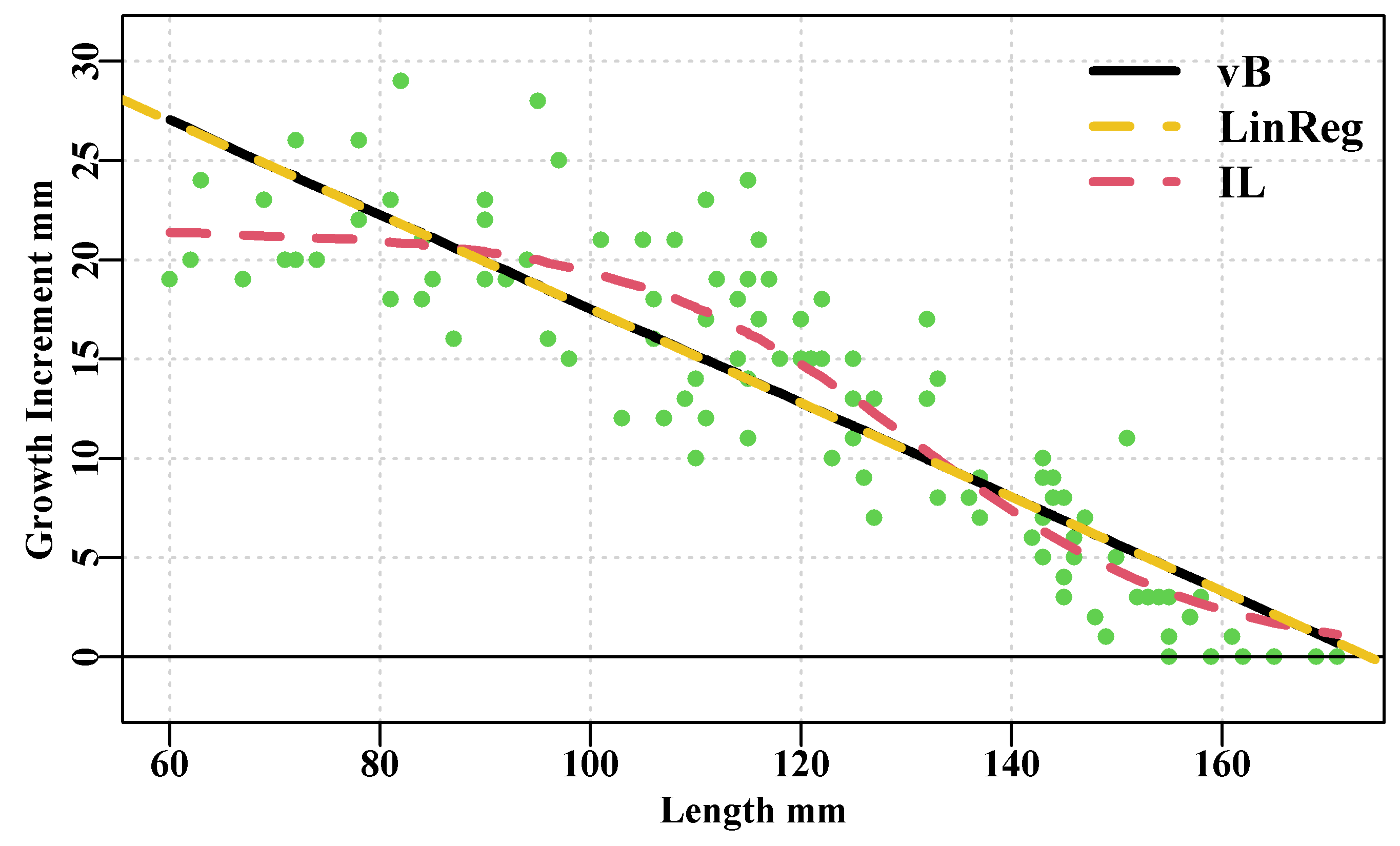
Figure 5.4: The von Bertalanffy (black), inverse logistic (curved dashed red), and linear regression (dashed yellow) fitted to blacklip abalone tagging data from Black Island. The time interval between tagging and recapture was 1.02 years. Obviously the vB and linear regression are identical.
The residuals of the two growth curves also exhibit the differences between the respective model fits.
 #residuals for vB and inverse logistic for tagging data Fig 5.5
parset(plots=c(1,2),outmargin=c(1,1,0,0),margin=c(.25,.25,.05,.05))
plot(bi$l1,(bi$dl - predvB),type="p",pch=16,col=1,ylab="",
     xlab="",panel.first=grid(),ylim=c(-8,11))
abline(h=0,col=1)
mtext("vB",side=1,outer=FALSE,line=-1.1,cex=1.2,font=7)
plot(bi$l1,(bi$dl - predil),type="p",pch=16,col=1,ylab="",
     xlab="",panel.first=grid(),ylim=c(-8,11))
abline(h=0,col=1)
mtext("IL",side=3,outer=FALSE,line=-1.2,cex=1.2,font=7)
mtext("Length mm",side=1,line=-0.1,cex=1.0,font=7,outer=TRUE)
mtext("Residual",side=2,line=-0.1,cex=1.0,font=7,outer=TRUE) 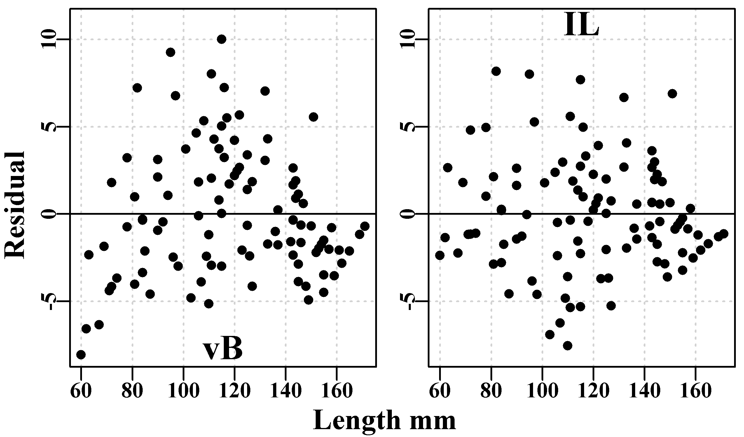
Figure 5.5: The von Bertalanffy (left hand) and inverse logistic (right hand) plots of the residuals from the curves fitted to blacklip abalone tagging data from Black Island. The time interval between tagging and recapture was 1.02 years.
5.3.4 A Closer Look at the Fabens Methods
The growth curve described by the Fabens transformation of the von Bertalanffy equation uses the same parameters but has smuggled in differences that are not immediately obvious. You will remember the example where we fitted the vB curve using two different residual error structures and that made the outcomes incomparable or, more strictly, incommensurate. The Fabens transformation has altered the residual structure and how the parameters interact with each other. Instead of the \(L_\infty\) being the average asymptotic maximum size it becomes the absolute maximum size, which is the reason it can predict negative growth increments. Strictly the parameters of the Faben’s model imply different things to that of the von Bertalanffy model.
We have compared the von Bertalanffy curve with the inverse-logistic but because we have used, as an example, data from an abalone stock we have obtained a rather biased view of which curve might be more useful. In most scalefish fisheries, the von Bertalanffy curve has been found to be most useful as a general description of growth, although it does have a few further problems. But a general problem with all growth models (not just tagging growth models) is the assumption that we have used so far, which is that the variation of the observations around the predicted growth trend will be constant. If we examine Figure(5.3) or Figure(5.4), and remember when we plotted the length-at-age data in the Model Parameter Estimation chapter, then in each case there are relatively clear trends in variation across either initial length or age. Instead of insisting on using a constant variance in the residuals (as required by SSQ), it is possible to use, for example, a constant coefficient of variation (\({\sigma}/{\mu}\)). If we used maximum likelihood methods it would be possible to have the variance of the residuals modelled separately allowing for a wide array of alternatives; Francis (1988) did exactly this. He fitted tagging models to data using maximum likelihood methods and assumed the residuals in each case were normally distributed, but he suggested a number of different functional forms for the relationship between residual variance and the expected \(\Delta L\) (functional relationships with the initial length are also possible). The approach we have used to date has assumed a constant variance so we have estimated a constant \(\sigma\) parameter. Instead, Francis (1988) suggested that the variance could have a constant multiplier between \(\sigma\) and \(\Delta L\), which would allow for an inverse relationship for tagging data. These considerations also apply to length-at-age models where the constant multiplier would allow for a linear relationship between age and \(\sigma\).
\[\begin{equation} \sigma = \upsilon (\Delta \hat{L}) \tag{5.5} \end{equation}\]
where \(\upsilon\) (upsilon) is a constant multiplier on the expected \(\Delta L\), and would need to be estimated separately. In such a case the normal likelihoods would become:
\[\begin{equation} L\left( \Delta L|Data \right)=\sum\limits_{i}{\frac{1}{\sqrt{2\pi }\upsilon \Delta \hat{L}}}\exp \left( \frac{{{\left( \Delta L-\Delta \hat{L} \right)}^{2}}}{2{{\left( \upsilon \Delta \hat{L} \right)}^{2}}} \right) \tag{5.6} \end{equation}\]
which describes the usual Normal likelihoods with \(\sigma^2\) replaced by \(( \upsilon \Delta \hat{L} )^{2}\). In addition to this simple alternative Francis (1988) also suggested, for tagging data, an exponentially declining residual standard deviation with a further estimable constant \(\tau\):
\[\begin{equation} \sigma = \tau \left( 1 - e^{-\upsilon (\Delta \hat{L})} \right) \tag{5.7} \end{equation}\]
Finally, Francis (1988) suggested a residual standard deviation that would be described by a power law:
\[\begin{equation} \sigma = \upsilon (\Delta \hat{L})^\tau \tag{5.8} \end{equation}\]
Francis (1988) also extended the Fabens approach to analyzing tagging data by considering the effect of bias, seasonal variation in growth rates, and the influence of outlier contamination. Often in the literature only a single aspect of a report is highlighted, which is one very good reason to always go back to the original literature rather than rely on a summary in another paper or book (like this one). Francis (1988) is an excellent place to start if you have to fit a growth curve to tagging data.
With each different formulation of the relationship between the variance of the residuals and the expected \(\Delta L\), the constants \(\tau\) and \(\upsilon\) would change in their interpretation. As seen before, the parameter estimates obtainable from the same model can vary if different error structures are assumed and they become incomparable. Unfortunately, how we select which error structure is most appropriate is not a question that is simple to answer. At very best, using non-constant variances will provide another view of the uncertainty associated with whichever curve is selected.
5.3.5 Implementation of Non-Constant Variances
By including a relationship between the expected \(\Delta L\) and the residual variance we would need to change the wrapper function around how the predicted values, \(\Delta \hat{L}\), were used to calculate the negative log-likelihood. Previously, with constant \(\sigma\) we used negNLL() so we could start by modifying that. All we have done is to include an extra function, funksig(), as an argument to negnormL() (see its help and code) thereby including the calculation of the sigma values. By doing this we could include a funksig() that retained a constant \(\sigma\), which would be a long version of the original negNLL(). But it also demonstrates that the function is behaving as expected. Then we can include an alternative funksig() that implements one of the three options above (or one of our own devising).
 # fit the Fabens tag growth curve with and without the option to
 # modify variation with predicted length. See the MQMF function
 # negnormL. So first no variation and then linear variation.
sigfunk <- function(pars,predobs) return(tail(pars,1)) #no effect
data(blackisland)
bi <- blackisland # just to keep things brief
param <- c(170.0,0.3,4.0); label=c("Linf","K","sigma")
modelvb <- nlm(f=negnormL,p=param,funk=fabens,funksig=sigfunk,
               indat=bi,initL="l1",delT="dt")
outfit(modelvb,backtran = FALSE,title="vB constant sigma",
       parnames = label)
# nlm solution: vB constant sigma
# minimum : 291.1691
# iterations : 24
# code : 1 gradient close to 0, probably solution
# par gradient
# Linf 173.9677972 9.565398e-07
# K 0.2653003 2.657143e-04
# sigma 3.5861240 1.391815e-05sigfunk2 <- function(pars,predo) { # linear with predicted length
sig <- tail(pars,1) * predo # sigma x predDL, see negnormL
pick <- which(sig <= 0) # ensure no negative sigmas from
sig[pick] <- 0.01 # possible negative predicted lengths
return(sig)
} # end of sigfunk2
param <- c(170.0,0.3,1.0); label=c("Linf","K","sigma")
modelvb2 <- nlm(f=negnormL,p=param,funk=fabens,funksig=sigfunk2,
indat=bi,initL="l1",delT="dt",
typsize=magnitude(param),iterlim=200)
outfit(modelvb2,backtran = FALSE,parnames = label,
title="vB inverse DeltaL, sigma < 1") # nlm solution: vB inverse DeltaL, sigma < 1
# minimum : 298.9086
# iterations : 46
# code : 1 gradient close to 0, probably solution
# par gradient
# Linf 170.9979114 -1.598948e-07
# K 0.2672788 1.488722e-06
# sigma 0.3941672 9.094947e-07Remember that by altering the residual structure the likelihoods become incommensurate and so we cannot determine which provides the better fit. The constant variance allowed the von Bertalanffy curve to stay effectively above the data at lengths greater than about 148, the changing variance growth curve was still mostly above the data but was being pushed closer to the later data by the reducing variance with predicted length. One could experiment by re-writing negnormL() to work with the initial lengths rather than predicted lengths. As indicated earlier separating the mean predicted lengths from the associated variance leads to great flexibility.
 #plot to two Faben's lines with constant and varying sigma Fig 5.6
predvB <- fabens(modelvb$estimate,bi)
predvB2 <- fabens(modelvb2$estimate,bi)
parset(margin=c(0.4,0.4,0.05,0.05))
plot(bi$l1,bi$dl,type="p",pch=1,cex=1.0,col=1,ylim=c(-2,31),
     ylab="Growth Increment mm",xlab="Length mm",panel.first=grid())
abline(h=0,col=1)
lines(bi$l1,predvB,col=1,lwd=2)         # vB
lines(bi$l1,predvB2,col=2,lwd=2,lty=2)  # IL
legend("topright",c("Constant sigma","Changing sigma"),lwd=3,
col=c(1,2),bty="n",cex=1.1,lty=c(1,2)) 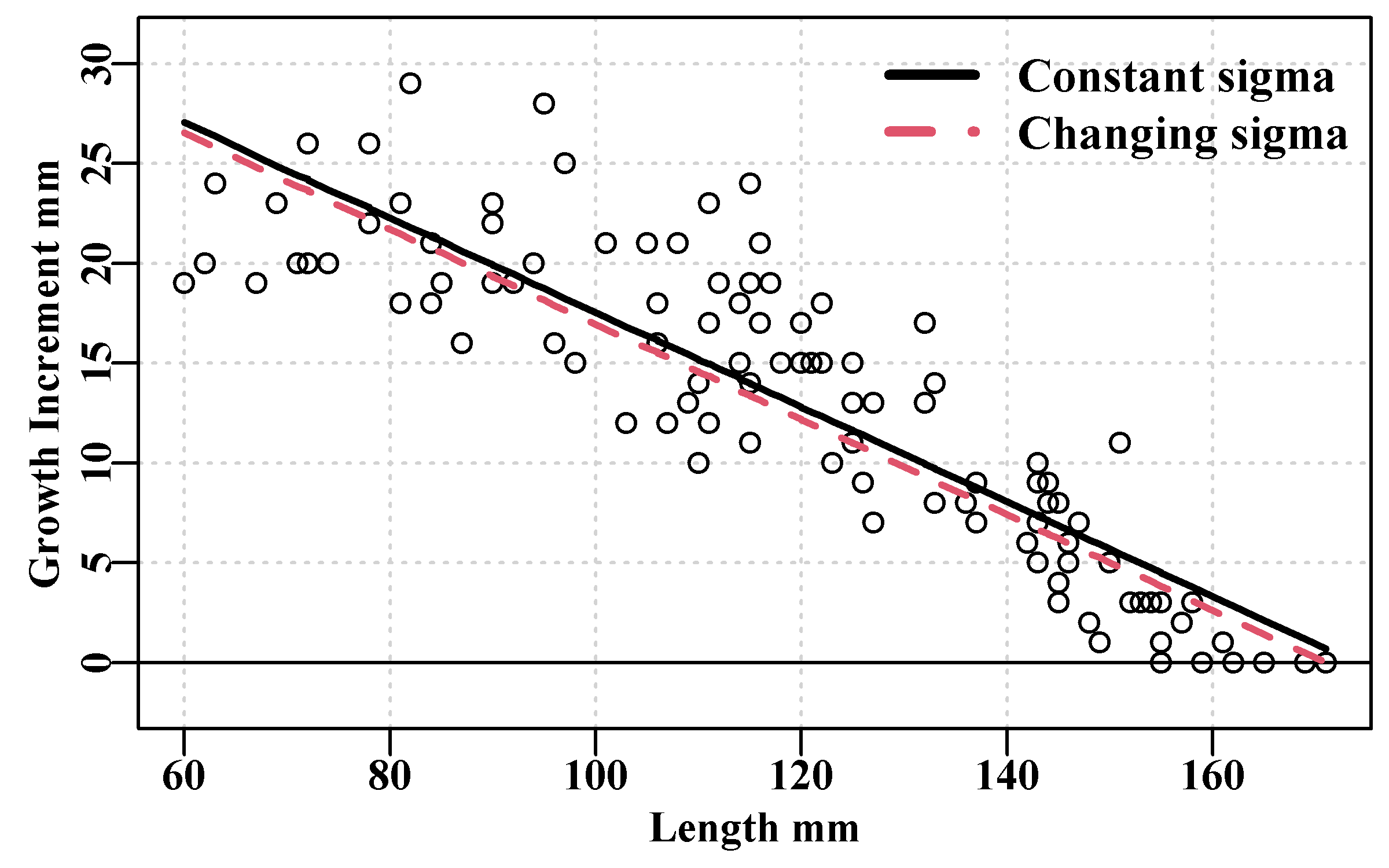
Figure 5.6: The von Bertalanffy (royal blue) with constant sigma, and the same but with sigma related to the changing DeltaL (red dashed) fitted to blacklip abalone tagging data from Black Island. The mean time interval between tagging and recapture was 1.02 years.
Our eyes are accustomed to appreciating symmetry and so the changing variation line in Figure(5.6) appears to be a relatively poor fit. But as a reflection of fitting a model assuming error only on the y-axis (the y-on-x issue) and with changing variances on the residuals, the lower dashed red line makes sense of data that has an intrinsic curve within its values. Using the more complex residual structure makes the model fitting more sensitive to initial conditions. You will have noticed that in the output the assumption of constant residual variance only took between 20 - 30 iterations, while with the functional relationship on the variance it took twice as many iterations (and that was with using the typsize optional argument to enhance stability, not used in the simpler model). If you modify those starting values you can easily obtain implausible answers.
Once again there needs to be good reasons for introducing such complexities into the modelling, although a changing variance tends to be clearly apparent when using length-at-age data, especially with the very young ages.
5.4 Objective Model Selection
In the chapter on Model Parameter Estimation we saw a similarly named section where an information theoretical approximation for the Akaike’s Information Criterion (AIC ; Akaike, 1974) based on sum-of-squares was presented (Burnham and Anderson, 2002). Now we are using maximum likelihood we will introduce the original version of the AIC as well as a discussion of likelihood ratios.
5.4.1 Akaike’s Information Criterion
The trade-off between the number of parameters used and the quality of a model’s fit to a data set is always an issue when selecting which model to use when attempting to describe a pattern in a data set. The classical approach is to select the simplest model that does a sufficiently good job of that description (Occam’s razor is simply an exhortation towards parsimony so if two models produce equivalent results select the simplest one). But how close is meant by “equivalent results” and what does “simplest” mean anyway. Akaike’s (1974) solution was to use a combination of the likelihoods and the “number of independently adjusted parameters within the model”. The AIC is a penalized likelihood based criteria for model selection where the smallest AIC indicates the optimum model (in terms of likelihood balanced against the number of parameters).
\[\begin{equation} AIC = -2\log{(L)} + \alpha p \tag{5.9} \end{equation}\]
where \(\log{(L)}\) is the total log-likelihood, \(p\) is the number of parameters explicitly varied when fitting the model, and \(\alpha\) is a multiplier (the penalty in penalized likelihood) whose value Akaike (1974) set to 2.0, using an argument from information theory. The emphasis on “independently adjusted parameters” that are “explicitly varied” is made to avoid confusion over model parameters which are held constant or which are derived from other parameters and model variables (we will see an example with the catchability parameter in surplus production models). For example, a common assumption in fishery models is that natural mortality, often depicted as \(M\), is a constant. As such it would not count in the AIC’s \(p\) value. The explicit identification of \(\alpha\) for the penalty rather than just putting a constant value of 2.0 has been made here to emphasize that there has been debate (Bhansali and Downham, 1977; Schwartz, 1978; Akaike, 1979; Atkinson, 1980) over the exact value that should be used to ensure that the balance between model complexity (number of parameters) and quality of fit (maximum likelihood or minimum sum of squares) reflects reality in simulations. The admittedly relatively dense statistical arguments tend to boil down to how large should the value of \(\alpha\), the penalty on \(p\), become? The outcome eventually became known as Schwartz’s Bayesian Information Criterion or, more briefly, the BIC.
\[\begin{equation} BIC = -2\log{(L)} + \log{(n)}p \tag{5.10} \end{equation}\]
where \(n\) is the sample size or number of data points to which the model with \(p\) parameters is fitted. As long as the number of data points is 8 or greater (\(log(8) = 2.079\)) then the BIC will penalize complex models more than AIC. On the other hand, intuitively, it makes sense to take some account of the sample size. If we apply these statistics to the comparison of the von Bertalanffy and inverse-logistic model fits that used constant \(\sigma\) estimates, Figure(5.4), using the MQMF function aicbic(), the inverse-logistic has both a smaller AIC and BIC and so would be the preferred model in this case.
 #compare the relative model fits of Vb and IL
cat("von Bertalanffy \n")
aicbic(modelvb,bi)
cat("inverse-logistic \n")
aicbic(modelil,bi)
# von Bertalanffy
# aic bic negLL p
# 588.3382 596.3846 291.1691 3.0000
# inverse-logistic
# aic bic negLL p
# 562.0244 572.7529 277.0122 4.00005.4.2 Likelihood Ratio Test
An alternative comparison between different model fits vs complexity can be made using what is known as a generalized likelihood ratio test (Neter et al, 1996). The method relies on the fact that likelihood ratio tests asymptotically approach the \(\chi^2\) distribution as the sample size gets larger. This means that with the usual extent of real fisheries data, this method is only approximate. Likelihood ratio tests are, exactly as their name suggests, the log of a ratio of two likelihoods, or if dealing directly with log-likelihoods, the subtraction of one from another, the two are equivalent (of course the likelihoods must be from the same PDF). We want to determine if either of two models, that use the same data and residual structure but different model structures (different parameters), provide for a significantly better model fit to the available data. As the likelihood ratio can be described by the \(\chi^2\) distribution it is possible to answer that question formally. Thus, for the likelihoods of two models, having either equal numbers of parameters or only one parameter difference, to be considered significantly different their ratio would need to be greater than the \(\chi^2\) distribution for the required number of degrees of freedom (the number of parameters that are different).
\[\begin{equation} \begin{split} -2 \times log{\left[ \frac{L(\theta)_{a}}{L(\theta)_b} \right]} &\le \chi _{1,1-\alpha }^{2} \\ -2 \times \left [LL(\theta)_a - LL(\theta)_b \right] &\le \chi _{1,1-\alpha }^{2} \end{split} \tag{5.11} \end{equation}\]
where \(L(\theta)_x\) is the likelihood of the \(\theta\) parameters for model \(x\), and \(LL(\theta)_x\) is the equivalent log-likelihood. \(\chi _{1,1-\alpha }^{2}\) is the \(1 - \alpha\)th quantile of the \(\chi^2\) distribution with 1 degree of freedom (e.g., for 95% confidence intervals, \(\alpha = 0.95\) and \(1 – \alpha = 0.05\), and \(\chi _{1,1-\alpha }^{2} = 3.84\).
In brief, if we are comparing two models that only differ by one or no parameters then if their negative log-likelihoods differ by more than 1.92 (3.84/2) then they can be considered to be significantly different and one will provide a significantly better fit than the other. If there were two-parameters different between the two models, then the minimum difference between their respective negative log-likelihoods for the models to differ significantly would need to be 2.995 (5.99/2) = \(\chi_{2,0.95}^2 /2\); two degrees of freedom), and so on for greater numbers of parameter differences (Venzon and Moolgavkar, 1988).
With respect to the comparison of the von Bertalanffy and inverse-logistic curves, the inverse-logistic negative log-likelihood is \(-2.0 \times (277.0122 - 291.1691) = 28.3138\), which is significantly smaller than that for the von Bertalanffy curve. We can use the MQMF function likeratio() to illustrate that this constitutes a highly significant difference between their respective fits to the data.
 # Likelihood ratio comparison of two growth models see Fig 5.4
vb <- modelvb$minimum # their respective -ve log-likelihoods
il <- modelil$minimum
dof <- 1
round(likeratio(vb,il,dof),8)
# LR P mindif df
# 28.31380340 0.00000005 3.84145882 1.000000005.4.3 Caveats on Likelihood Ratio Tests
Given the prevalence of using weighted log-likelihoods in fishery models, when using a likelihood ratio test to compare alternative models one needs to be careful that the models are in fact comparable. When we are using the same data and the same probability density function to describe the residual distribution then we can use a likelihood ratio test. But remember the example where we compared the application of the same growth model to the same data only with a different assumption regarding the residual error structure (log-normal rather than normal). Those curves were simply incomparable (incommensurate). Similarly with penalized likelihoods where different weightings may be given to particular data streams in different model versions, such changes make the models incommensurate It sounds obvious that one should only compare comparable models, but sometimes, with some of the more complex models determining what constitutes a fair comparison is not always simple.
5.5 Remarks on Growth
Description of individual growth processes are important to fishery models because the growth in size and weight of individuals is a major aspect of the productivity of a given stock. This growth is obviously one of the positives in the balance between those processes that increase a stock’s biomass and those that decrease it. But it is important to understand that invariably the descriptions of growth are only descriptions and are useful primarily across the range of sizes for which we have data. There are many instances where the weaknesses relating to the extrapolation of the von Bertalanffy curve lead to biologically ridiculous predictions (Knight, 1968). But such instances are mistaking a particular interpretation of the model’s parameters for reality, whereas the curve is merely a description of the growth data and is strictly only valid across where there are data. This is one reason why growth model transformations have been produced that then have estimated parameters that can be located within the range of the available data (Schnute, 1981; Francis, 1988, 1995).
5.6 Maturity
5.6.1 Introduction
Fisheries management now tends to use what are known as biological reference points to form the foundation of what it hopes constitutes rational and defensible management decisions for harvested renewable natural resources (FAO, 1995, 1996, 1997; Restrepo and POwers, 1999; Haddon, 2007). Put very simply the idea is to have a target reference point, which is very often defined as a mature or spawning biomass level, or some proxy for this, that is deemed a desirable state for the stock. It is desirable because, generally, it ought to provide for good levels of subsequent recruitment and provide the stock with sufficient resilience to withstand occasional environmental shocks. Common default values can be \(B_{40}\), meaning \(40\%B_0\), or a depletion level of 40%, which is used as a proxy for \(B_{MSY}\), or the spawning biomass that can sustainably produce the maximum sustainable yield. In Australia, the Commonwealth Harvest Strategy Policy defines the target as \(B_{48}\), which is used as a proxy for \(B_{MEY}\), or the spawning biomass that should be capable of producing the maximum economic yield (note it is the biomass level, \(B_{MEY}\), that is the target not the \(MEY\); DAFF, 2007; Rayns, 2007). In addition, one defines a limit reference point, again in terms of a level of mature biomass (or proxy) below which the stock concerned would be deemed to be at risk of its recruitment being compromised. Biological reference points are often couched in terms relative to an estimate of what the unfished spawning biomass would be (\(B_0\)). The concept of \(B_0\) can be either an equilibrium notion or a more dynamic version that attempts to account for recruitment variation. Whatever the case this number tends to be uncertain within assessments and also often changes between assessments (Punt et al, 2018). To produce management advice one needs three things:
an assessment of what the current stock status is, in terms of spawning biomass depletion, and hence
the current estimate of unfished spawning biomass, and finally
a harvest control rule that determines what fishing mortality , effort, or catch will be allowed in the next season(s).
Perhaps you have noticed I am using the terms mature and spawning biomass inter-changeably. By doing this I am not trying to confuse you but rather trying to inure you to the varying terminology you will come across in the literature.
The emphasis on mature or spawning biomass is the reason that obtaining a reasonable estimate of the size- or age-at-maturity is so important. It is so that any estimate of how much mature biomass there is reflects the biology of the stock as well as the current state of the fishery. In this book we are trying to stay focussed on the modelling but it is always the case that we are trying to model an underlying biological reality. In fact, the biological reality, rather like the details of growth, is often rather complex. In fisheries theory many of the foundations derive from the northern hemisphere, and especially from working on highly productive stocks in the North Sea and the Atlantic (Smith, 1994). Many of the commercial species there have relatively simple reproductive histories. There are males and females that, as a population, mature to an average schedule, they spawn either once or each year until they die. That is, of course, an over-simplification, and the biological world is much more varied than that, even in the northern hemisphere. There are species that all start off as females with some of the larger females turning into males (protogynous), and vice versa (protandrous). There are many different reproductive strategies out there and many of them can influence things like the size and/or age at maturity. However, here we will focus only on the classical approach. Nevertheless, with your own examples, do not make assumptions about biology, it is always the case that representative evidence from a population is better than assumptions.
The size- or age-at-maturity is a population property. Individuals may undergo a process of maturation and take time to become capable of spawning, but the process we are describing is taken as an average across a population. Given a sample, hopefully a large sample that adequately bridges the size- or age-at-maturity, we are aiming to describe the proportion of fish that are mature at each size or age. The concept of size-at-maturity is often summarized as being the size at which 50% of a population are considered to be mature (capable of spawning). In fact, \(Lm_{50}\), the size at 50% maturation, is only part of the what is important, in addition, as we shall see, some measure of how quickly a species matures with respect to size or age is also important. Some simpler fisheries models still use an assumption of what is known as knife-edge maturity, which implies the strong assumption that 100% of animals become mature at a given age. We will discuss how the time taken for the population to mature affects the population dynamics later. How one determines maturity will not be considered here, though ideally one uses histology to confirm maturing gametes rather than simply using a visual inspection of fish gonads. Once again, there is a huge literature devoted to the details of determining maturity stages in a wide range of species, but we will not attempt to approach that. The task we have is finding a mathematical description of the expected population maturation curve. And the expectation is that the proportion of animals considered mature will increase with size and age until 100% are mature (though there are exceptions even to this, with the females of some species taking some years off from reproduction to recover from the large energy investment they make to the generation of eggs). Life history characteristics come into this in terms of whether a species is adapted to breed once (semelparity) or many times (iteroparity), or whether it generates vast numbers of small eggs or far fewer large eggs, or even produce a few live young. Always remember that biology can be complex and mathematical descriptions of biology are relatively simple abstractions.
5.6.2 Alternative Maturity Ogives
The general pattern of maturation within a population is that maturation will be found across a range of sizes and ages, with a proportion maturing both early and late, and most maturing around some average time. If we imagine some sort of parabolic curve of the proportion maturing through time, possibly close to normal but with shorter tails, what we want is the cumulative density function of that distribution running from 0 to 100% across some range of sizes or ages. The outcome is an S-shaped curve commonly called a logistic curve and in the literature there are a remarkable number of different mathematical representations of such curves. The statistics of interest are the \(Lm_{50}\) (the size/age at 50% maturity), and the \(IQ\), the inter-quartile distance that measures the range of sizes/ages between the 25th and 75th quartiles of the maturity ogive (at what age are 25% and 75% mature). The use of the inter-quartile range is an arbitrary choice but reflects common practice (as seen in boxplots), but does not preclude using a wider or a narrower range if those are convenient.
Among the many different versions available there is a classical logistic curve, Equ(5.12), commonly used to describe maturation in many populations (see the MQMF function mature()). This formulation lends itself easily to being fitted using a Generalized Linear Model with Binomial errors. We have been using R as a programming environment but here is a chance to remember that its first purpose was to act as a tool for statistical analyses.
\[\begin{equation} p_L \;\; = \;\; \frac{exp(a + bL)}{1 + exp(a + bL)} \;\; =\;\; \frac{1}{1+exp(a+bL)^{-1}} \tag{5.12} \end{equation}\]
\(p_L\) is the proportion mature at length \(L\), and \(a\) and \(b\) are the exponential parameters. Notice I have not included an error term in the equation. Here we are attempting to make predictions about mature or not mature observations related to different sizes (for brevity I will stop writing ‘size or age’ each time). This is what suggests that we should be using Binomial errors, as described in the Model Parameter Estimation chapter. Another nice thing about this formulation is that the \(Lm50 = -a/b\), that is the size at 50% maturity is simply derived from the parameters. Similarly, the inter-quartile distance can also be derived from the parameters as \(IQ=2 \times log(3)/b = 2.197225 \times b\).
Maturity data is Binomial in nature, at a given time of sampling a population, the observations are whether each sampled fish, of size \(L\), is mature or not. The book’s R package, MQMF contains an example data set for us to work with, tasab, which includes blacklip abalone (Haliotis rubra) data from two sites along a 16km stretch of Tasmanian coastline.
 # The Maturity data from tasab data-set
data(tasab)       # see ?tasab for a list of the codes used
properties(tasab) # summarize properties of columns in tasab
# Index isNA Unique Class Min Max Example
# site 1 0 2 integer 1 2 1
# sex 2 0 3 character 0 0 I
# length 3 0 85 integer 62 160 102
# mature 4 0 2 integer 0 1 0#
# F I M
# 1 116 11 123
# 2 207 85 173Abalone are notorious (infamous!) for being highly variable in their biological characteristics across relatively small spatial scales, so the fine detail of sampling site is important (Haddon and Helidoniotis, 2013). This data was all collected in the same month and year by the same people so the only factor other than shell length that we might think could influence maturation would be the specific site (the sexes appear to mature at the same time and sizes; Figure(5.7)).
 #plot the proportion mature vs shell length  Fig 5.7
propm <- tapply(tasab$mature,tasab$length,mean) #mean maturity at L
lens <- as.numeric(names(propm))            # lengths in the data
plot1(lens,propm,type="p",cex=0.9,xlab="Length mm",
ylab="Proportion Mature") 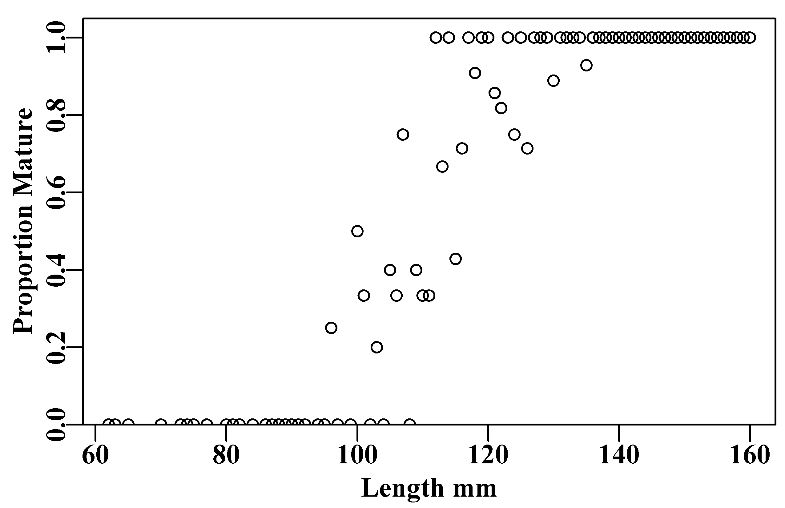
Figure 5.7: The proportion mature at length for the blacklip abalone maturity data in the tasab data set.
The data appear relatively noisy, although this is difficult to appreciate as some of the observed lengths whose proportion mature was neither 0 nor 1, may have had only a few observations. For example, there is a single point lined up on a proportion mature of 0.5 at length 100mm, and if you delve into the data you will find that that point is only made up of two observations, one mature the other not. One can find the lengths with pick <- which(tasab$length == 100), or which(propm == 0.5), and then use tasab[pick,] to see the data.
Examining the data set using properties(tasab) or head(tasab,10), tells us what variable names we are dealing with. While we obviously want to examine the relationship between the variables mature and length, remember that initially we also want to examine the influence of site on maturation. Importantly, we need to convert the site variable into a categorical factor otherwise it will be treated as a vector of the integers 1 and 2, rather than as potentially different treatments. We cannot include sex as a factor as it has more than two outcomes in that all animals start out as Immature, although one can always analyse the male and female data separately. However, over many more sites, no repeatable differences in the rate or mean size at maturity x site have been found, so far, between the sexes in blacklip abalone. Once fitted we will see that site is uninformative to the analysis (it is insignificant) and so we repeat the analysis without site.
 #Use glm to estimate mature logistic
binglm <- function(x,digits=6) { #function to simplify printing
  out <- summary(x)
  print(out$call)
  print(round(out$coefficients,digits))
  cat("\nNull Deviance  ",out$null.deviance,"df",out$df.null,"\n")
  cat("Resid.Deviance ",out$deviance,"df",out$df.residual,"\n")
  cat("AIC  = ",out$aic,"\n\n")
  return(invisible(out)) # retain the full summary
} #end of binglm
tasab$site <- as.factor(tasab$site) # site as a factor
smodel <- glm(mature ~ site + length,family=binomial,data=tasab)
outs <- binglm(smodel)  #outs contains the whole summary object

model <- glm(mature ~ length, family=binomial, data=tasab)
outm <- binglm(model)
cof <- outm$coefficients
cat("Lm50 = ",-cof[1,1]/cof[2,1],"\n")
cat("IQ   = ",2*log(3)/cof[2,1],"\n")
# glm(formula = mature ~ site + length, family = binomial, data = tasab)
# Estimate Std. Error z value Pr(>|z|)
# (Intercept) -19.797096 2.361561 -8.383056 0.000000
# site2 -0.369502 0.449678 -0.821703 0.411246
# length 0.182551 0.019872 9.186463 0.000000
#
# Null Deviance 564.0149 df 714
# Resid.Deviance 170.7051 df 712
# AIC = 176.7051
#
# glm(formula = mature ~ length, family = binomial, data = tasab)
# Estimate Std. Error z value Pr(>|z|)
# (Intercept) -20.464131 2.265539 -9.032787 0
# length 0.186137 0.019736 9.431291 0
#
# Null Deviance 564.0149 df 714
# Resid.Deviance 171.3903 df 713
# AIC = 175.3903
#
# Lm50 = 109.9414
# IQ = 11.80436In the first analysis, that included site, because I made sure that the sites included were similar when putting the data together, site 2 was not significantly different from site 1 (P=0.411), implying that, in this case, the site factor was not informative for this analysis. The analysis was thus repeated omitting site from the equation. Had the sites exhibited significant differences then we would require multiple curves to describe the model results. We will plot them as different curves anyway to illustrate the process. The extra site parameters are modifiers to the initial exponential intercept value. Thus, the ab$length parameter is the \(b\) parameter in both cases, but the curve for site 1 would be obtained by treating the intercept as the \(a\) parameter and the curve for site 2 would require us to add the parameter values for the intercept and ab$site2 as the \(a\) parameter. Thus, site1 model \(a=-19.797\) and \(b=0.18255\), while for site2 model \(a=-19.797-0.3695\) and \(b=0.18255\). Adding the final no-site model to the plot indicates that the combined model is closer to site 2, which is a reflection of the fact that the number of observations at site 2 was 465 while only 250 at site 1. Note that with one parameter less the residual deviance is very slightly greater but despite this the AIC for the simpler model is smaller than that for the model including site as a factor, which again reinforces the idea that the simpler model provides an improved balance between complexity and model fit. There are obvious analogies with General Linear Models and their comparisons and manipulations. If one does find a significant difference between the intercepts then it would be sensible to test whether the difference also extended to the \(b\) parameter to determine whether the curves needed to be treated completely separately. Sharing common parameters is often helpful as it leads to increases in sample size.
 #Add maturity logistics to the maturity data plot Fig 5.8
propm <- tapply(tasab$mature,tasab$length,mean) #prop mature
lens <- as.numeric(names(propm))       # lengths in the data
pick <- which((lens > 79) & (lens < 146))
parset()
plot(lens[pick],propm[pick],type="p",cex=0.9, #the data points
      xlab="Length mm",ylab="Proportion Mature",pch=1)
L <- seq(80,145,1) # for increased curve separation
pars <- coef(smodel)
lines(L,mature(pars[1],pars[3],L),lwd=3,col=3,lty=2)
lines(L,mature(pars[1]+pars[2],pars[3],L),lwd=3,col=2,lty=4)
lines(L,mature(coef(model)[1],coef(model)[2],L),lwd=2,col=1,lty=1)
abline(h=c(0.25,0.5,0.75),lty=3,col="grey")
legend("topleft",c("site1","both","site2"),col=c(3,1,2),lty=c(2,1,4),
lwd=3,bty="n") 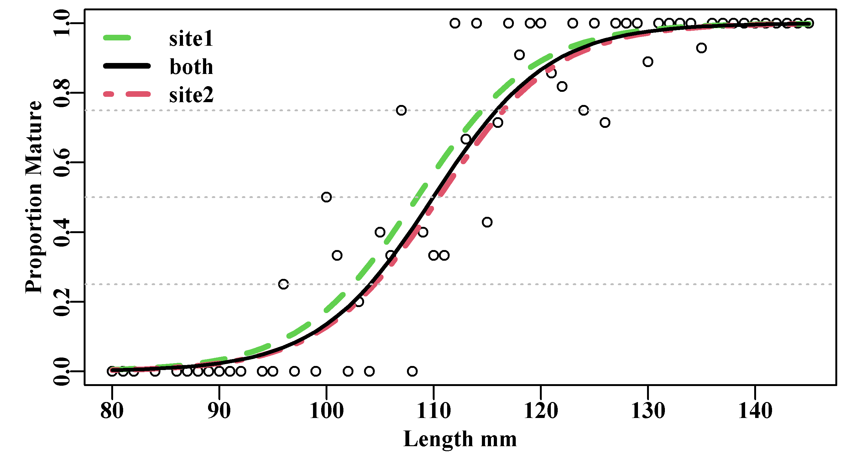
Figure 5.8: Proportion mature at length for blacklip abalone maturity data (tasab data-set). The combined analysis, without site (both) is closer to site 2 (dot-dash) than site 1 (dashes), which reflects site 2’s larger sample size.
Large sample sizes often improve the quality of the model fit. With sufficient data it may be the case that the variability currently exhibited by the data would be sufficiently reduced that a statistically significant difference could be found between these sites. However, if we consider that the difference between the \(Lm_{50}\) for site 1 and site 2 is about 2 mm (out of 110), then biologically, such a difference may not be important as other factors such as growth between the two sites may also vary. As with any model or statistical analyses the biological implications should be taken into account in addition to being concerned about statistical significance.
5.6.3 The Assumption of Symmetry
In very many instances the standard logistic curve does a fine job of describing a transition from immature to mature (or maybe some other biological transition, such as cryptic to emergent, moult stage A to stage B, etc). However, a major restriction of the classical logistic is that it is symmetric around the \(L_{50}\) point, which may not be an optimum description for real world events.
An array of alternative asymmetric curves have been suggested but fortunately, a general or unified model for the description of “fish growth, maturity, and survivorship data” was proposed by Schnute and Richards (1990) and this generalizes the classical logistic model used for maturity as well the growth models by Gompertz (1825), von Bertalanffy (1938), Richards (1959), Chapman (1961), and Schnute (1981), some of which can also be used to describe maturation.
The Schnute and Richards (1990) model has four parameters:
\[\begin{equation} y^{-b} = 1 + \alpha \; exp(-a \;x^c) \tag{5.13} \end{equation}\]
which can be re-arranged, Equ(5.14), to better illustrate the relationship with the classical logistic curve, Equ(5.12), which, if we set both \(b = c = 1.0\) would be equivalent to the classical logistic (e.g. set \(\alpha = 300\), and \(a = 0.12\)):
\[\begin{equation} y = \frac {1}{\left( 1 + \alpha \; exp(-a \; x^c \right)^{1/b}} \tag{5.14} \end{equation}\]
If one of the special classical cases is used it may be that there are analytical solutions for determining the \(L_{50}\) and the \(IQ\) but otherwise they would need to be found numerically (see the MQMF functions bracket() and linter()). This curve can be fitted to maturity data using Binomial errors as before, although using nlm() or some other non-linear solver (Schnute and Richards, 1990, provide the required likelihoods). But it is likely that the special cases might provide more stable solutions to the full four parameter model. The asymmetry of the possible curves from (Equ(5.14)) is easily demonstrated using the MQMF srug() function (Schnute and Richards Unified Growth). In the absence of an analytical solution to finding the \(L_{50}\) and \(IQ\) we can use the two functions bracket() and linter(), which bracket the target values (in this case 0.25, 0.5, and 0.75) and then linearly interpolate to generate an approximate estimate of the required statistics (see their help files and examples).
 #Asymmetrical maturity curve from Schnute and Richard's curve Fig5.9
L = seq(50,160,1)
p=c(a=0.07,b=0.2,c=1.0,alpha=100)
asym <- srug(p=p,sizeage=L)
L25 <- linter(bracket(0.25,asym,L))
L50 <- linter(bracket(0.5,asym,L))
L75 <- linter(bracket(0.75,asym,L))
parset()
plot(L,asym,type="l",lwd=2,xlab="Length mm",ylab="Proportion Mature")
abline(h=c(0.25,0.5,0.75),lty=3,col="grey")
abline(v=c(L25,L50,L75),lwd=c(1,2,1),col=c(1,2,1)) 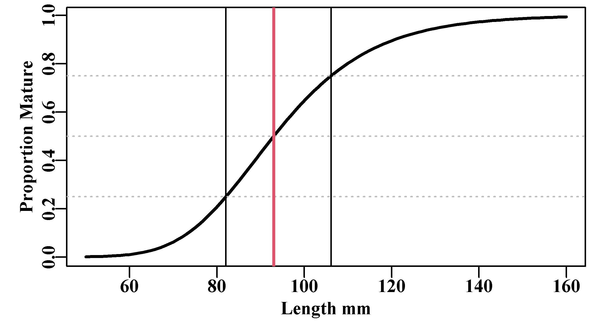
Figure 5.9: The proportion mature at length for a hypothetical example using the Schnute and Richards unified growth curve. The asymmetry of this logistic curve is illustrated by the difference between the left and right hand sides of the inter-quartile distance shown by the green lines.
Using the same parameters used in Figure(5.9) as a baseline, we can vary the individual parameters separately to determine the effect upon the resulting curves. The \(a\) and \(c\) parameters are relatively influential on the inter-quartile distance and all four are influential on the \(L_{50}\).
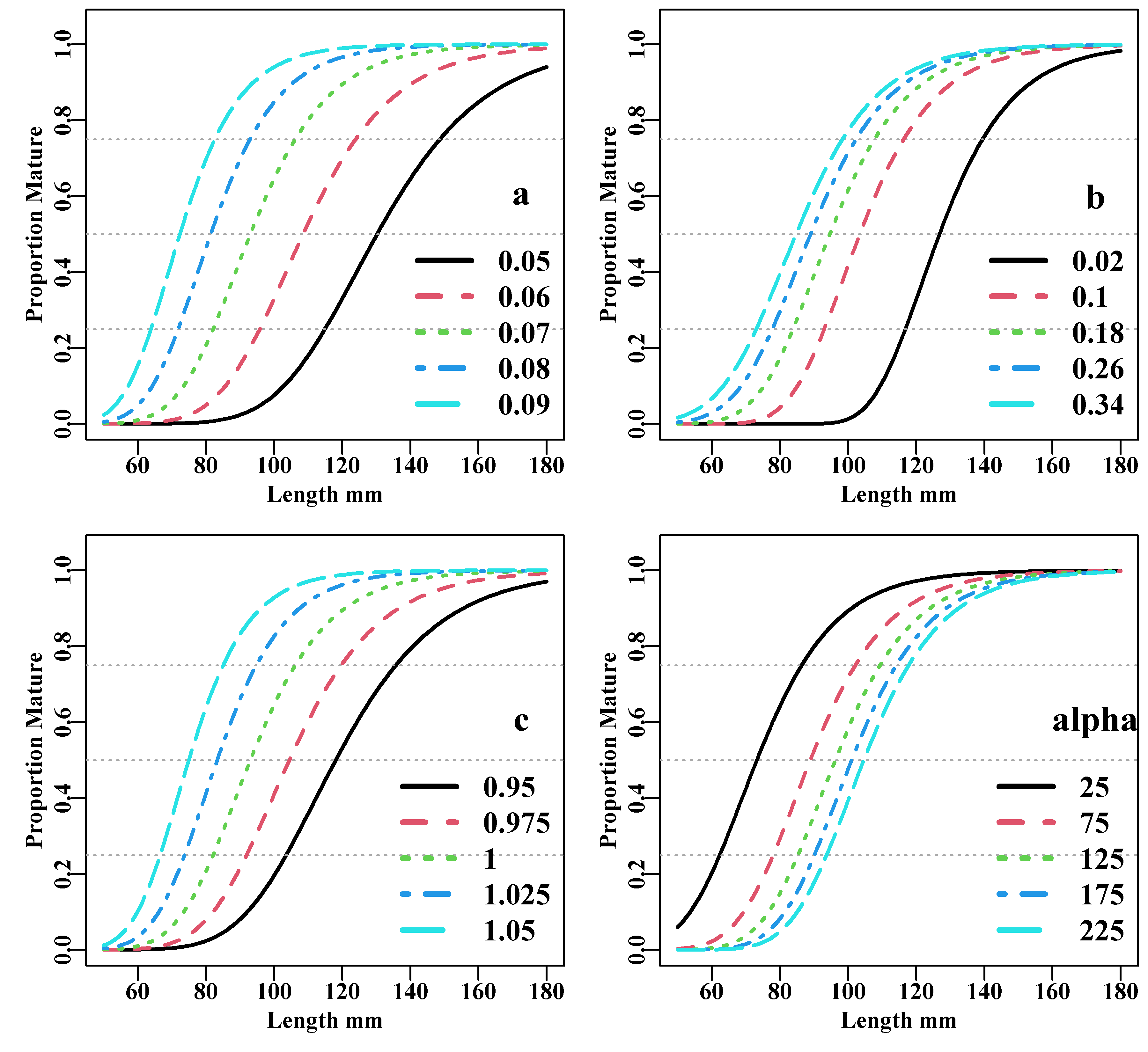
Figure 5.10: The proportion mature at length for hypothetical examples using the Schnute and Richards unified growth curve. The parameters when not varying were set at a=0.07, b=0.2, c=1.0, and alpha=100.
Schnute’s (1981) model appears to have been used more in the literature than the more general Schnute and Richards (1990) model, but this is natural when the intent of the Schnute and Richard’s model is to demonstrate that all these different curves can be unified and thus share a degree of commonality. This emphasizes that these curves provide primarily empirical descriptions of biological processes, which themselves are emergent properties of the populations being studied. Providing strict biological interpretations of their parameters and expecting nature to always provide for plausible or sensible parameter values is an extrapolation too far. An example is the situation described by Knight (1968), who was writing about growth but really discussing the reality or otherwise of giving explicit interpretations to the parameters of empirical models. He stated: “More important is the distorted point of view engendered by regarding \(L_{\infty}\) a fact of nature rather than as a mathematical artifact of the data analysis.” (Knight, 1968, p 1306). Models which are descriptive rather than explanatory (hypothetical about a process) remain empirical descriptions and care is needed when trying to interpret their parameters.
5.7 Recruitment
5.7.1 Introduction
The main contributors to the production of biomass within a stock are the recruitment of new individuals to a population and the growth of individual (where the definition of a stock means we need not consider immigration). Once again there is a huge literature on recruitment processes (Cushing, 1988; Myers and Barrowman, 1996; Myers, 2001), but here we will focus mainly on how it is described when attempting to include its dynamics within a model. As with other static models of growth and maturity such models are assumed to remain constant through time, although the option exists within stock assessment models of time-blocking different parameter sets within particular delineated time periods (Wayte, 2013). Here we will focus on the simple descriptions.
Recruitment to fish populations naturally tends to be highly variable, with the degree of variation varying among species. If you think I am using the term variation and related terms too often in a single sentence, perhaps that will reinforce the notion that recruitment really is highly variable. The main problem for fisheries scientists is whether recruitment is determined by the spawning stock size or environmental variation or some combination of both. This harks back to the debate in population dynamics from the 1950s about whether populations were controlled by density-dependent or density-independent effects (Andrewartha and Birch, 1954). This issue of variation has led to a commonly held but mistaken belief that the number of recruits to a fishery is effectively independent of the adult stock size over most of the observed range of stock sizes. This can be a dangerous assumption (Gulland, 1983). The notion of no recruitment relationship with spawning stock size suggests that scientists and managers can ignore stock recruitment relationships unless there is clear evidence that recruitment is not independent of stock size. The notion of no stock recruitment relationship existing derives from data on such relationships commonly appearing to be very scattered, with no obvious pattern.
Despite these arguments the modelling of recruitment processes has importance within fisheries models because when they are used to provide management advice forwards from the present, the model dynamics are often projected forwards while examining the effect of alternative harvest or effort levels. By including uncertainty in those projections it is possible to estimate the relative risk of alternative management arrangements failing to achieve desired management objectives (Francis, 1992). But to make such projections means having information about a stock’s productivity. Assuming that the dynamics of individual growth have been covered, estimates of a time series of recruitment levels or some defined stock recruitment relationship can be used to produce estimates of future recruitment levels for such projections.
In this chapter, we will consider only mathematical descriptions of stock recruitment relationships and mostly ignore the biology behind those relationships, although there are always exceptions. We will review just two of the most commonly used mathematical models of stock recruitment and will discuss their use in stock assessment models of varying complexity.
5.7.2 Properties of “Good” Stock Recruitment Relationships
A good introduction to the biological processes behind stock recruitment relationships is given by Cushing (1988), who provides an overview of the sources of egg and larval mortality along with good examples and a bibliography on the subject. As with the other fundamental production processes we have discussed, there is an enormous literature on the biology of stock recruitment relations and their modifiers.
A great variety of influences, both biological and physical, have been recorded as affecting the outcome of recruitment. We will not be considering the biological details of any real species except to point out that the relation between stock size and resulting recruitment is not deterministic, and there can be a number of forms of feedback affecting the outcome. Various mathematical descriptions of stock recruitment relationships have been suggested, but we will only consider those by Beverton and Holt and Ricker, but others such as that by Deriso-Schnute (Deriso, 1980; Schnute, 1985) are also important.
Ricker (1975) listed four properties of average stock recruitment relationships that he considered desirable:
A stock recruitment curve should pass through the origin; that is, when stock size is zero, there should be no recruitment. This assumes the observations being considered relate to the total stock, and that there is no “recruitment” made up of immigrants.
Recruitment should not fall to zero at high stock densities. This is not a necessary condition, but while declines in recruitment levels with increases in stock densities have been observed, declines to a zero recruitment index have not. Even if a population was at equilibrium at maximum stock biomass, recruitment should still match natural mortality levels.
The rate of recruitment (recruits-per-spawner) should decrease continuously with increases in parental stock. This is only reasonable when positive density-dependent mechanisms (compensatory) are operating (for example, an increase in stock leads to an increase in larval mortality). But if negative density-dependent mechanisms (depensatory) are operating (for example, predator saturation and Allee effects; Begon and Mortimer, 1986), then this may not always hold.
Recruitment must exceed parental stock over some part of the range of possible parental stocks. Strictly, this is only true for species spawning once before dying (e.g., salmon). For longer-lived, multi-spawning species, this should be interpreted as recruitment must be high enough over existing stock sizes to more than replace losses due to annual natural mortality.
Hilborn and Walters (1992) suggested two other general properties that they considered associated with good stock recruitment relationships:
The average spawning stock recruitment curve should be continuous, with no sharp changes over small changes of stock size. They are referring to continuity, such that average recruitment should vary smoothly with stock size, related to condition 3 above.
The average stock recruitment relationship is constant over time. This is stationarity, where the relationship does not change significantly through time. This assumption seems likely to fail in systems where the ecosystem, of which the exploited population is a part, changes markedly. But within models can be handled using time-blocks of parameters (for an example see Wayte, 2013).
5.7.3 Recruitment Overfishing
The term ‘overfishing’ is commonly discussed in two contexts, growth overfishing and recruitment overfishing. Growth overfishing is where a stock is fished so hard that eventually most individuals are caught at a relatively small size. This is a problem in terms of yield-per-recruit (YPR). The analysis of YPR focusses upon balancing stock losses due to total mortality against the stock gains from individual growth with an aim to determining the optimum size and age at which to begin harvesting the species (where optimum can take a number of meanings). Growth overfishing is where the fish are being caught before they have time to reach this optimal size.
Recruitment overfishing is said to occur when a stock is fished so hard that the spawning stock size is reduced below the level at which it, as a population, can produce enough new recruits to replace those dying (either naturally or otherwise). Obviously, such a set of circumstances could not continue for long, and sadly, recruitment overfishing is usually a precursor to fishery collapse. Although keep in mind that fishery collapse usually means that a fishery is no longer economically viable, it does not mean literal extinction.
While growth overfishing is relatively simple to detect (if the stock at YPR optimum or not? Although, of course, there can be complications). Unfortunately, the same cannot be said about the detection of recruitment overfishing, which could require a determination of the relation between mature or spawning stock size and recruitment levels. This has proven to be a difficult task for very many fisheries. Instead, it has become common, with the advent of formal harvest strategies, to identify a spawning biomass level deemed to constitute an unacceptable risk to subsequent recruitment. A very common limit reference point is taken to be 20% of unfished spawning biomass (\(0.2B_0\)). The earliest reference to a Limit Reference Point depletion level of \(20\%B_0\) appears to be Beddington & Cooke (1983). They explained a constraint they imposed on their analyses of potential yields from different stocks in the following manner:
“… an escapement level of 20% of the expected unexploited spawning stock biomass is used. This is not a conservative figure, but it represents a lower limit where recruitment declines might be expected to be observable.” (Beddington & Cooke, 1983, p9‐10).
The most influential document giving rise to the notion that \(B_{20\%}\) (note the different ways of depicting \(0.2B_0\)) is a reasonable depletion level to use as an indicator of potential recruitment overfishing was a document prepared for the National Marine Fisheries Service in the USA (Restrepo et al., 1998). In fact, they recommend \(0.5B_{MSY}\) but consider \(B20\%\) to be an acceptable proxy for that figure. However, it is important to note that this is only a ‘rule of thumb’ and there is no empirical basis that links the proxy \(B_{LIM} = B_{20\%}\) or to \(0.5B_{MSY}\). Indeed, selecting \(0.5B_{MSY}\) for some species could result in \(B_{LIM}\) much lower than \(B_{20\%}\).
5.7.4 Beverton and Holt Recruitment
Historically, Beverton and Holt’s (1957) stock recruitment curve was useful because of its simple interpretation, which also meant it could be derived from first principles. Being mathematically tractable was also important to them as, at the time, only analytical methods were feasible. In fact, its continued use appears to stem a great deal from inertia and tradition. You should note that if we are to treat the Beverton–Holt curve simply as a mathematical description, then effectively any curve, with the good properties listed earlier, could be used. One talks of “the” Beverton-Holt stock recruitment model, however, it comes in more than one form. There are two common forms used:
\[\begin{equation} R_y = \frac{B_{y-1}}{\alpha + \beta B_{y-1}}exp(N(0,\sigma_R^2)) \tag{5.15} \end{equation}\]
where \(R_y\) is the recruitment in year \(y\), \(B_y\) is the spawning biomass in year \(y\), \(\alpha\) and \(\beta\) are the two Beverton-Holt parameters, and \(exp(N(0,\sigma_R^2))\) represents the assumption that any relationship between predicted model values and observations from nature will be log-normally distributed (often represented as \(e^{\varepsilon}\)). The \(\beta\) value determines the asymptotic limit (\(= 1/\beta\)), while the differing values of \(\alpha\) are inversely related to the rapidity with which each curve attains the asymptote, thus determining the relative steepness (a keyword, which we will hear much more about) near the origin (the smaller the value of \(\alpha\), the quicker the recruitment reaches a maximum). Of course, this is an average relationship and the scatter about the curve is as important as the curve itself. A common alternative re-parameterized formulation is:
\[\begin{equation} R_y = \frac{aB_{y-1}}{b + B_{y-1}}e^{\varepsilon} \tag{5.16} \end{equation}\]
where \(a\) is the maximum recruitment (\(a = 1/\beta\)), and \(b\) is the spawning stock (\(b = \alpha/\beta\)) needed to produce, on average, half maximum recruitment (\(a/2\)). The use of \(y-1\) for the biomass that gives rise to the recruits in year \(y\) has implications for the time of spawning. If spawning occurs in December and settlement of larval forms occurs in the following year then this would be correct, if they both occurred in the same year then obviously the subscript would need changing. The thing to note is that biological reality, in this case relating to timing, can even creep into very simple models. Mathematical models can provide wonderful representations of nature but one needs to be aware of the biology of the animals being modelled to avoid simple mistakes!
It is clear from Figure(5.11) that the initial steepness of the Beverton–Holt curve along with the asymptotic value captures the important aspects of the behaviour of the equation. The asymptote is given by the value of the parameter \(a\), while the initial steepness is approximated by the value of (\(a/b = 1/\alpha\)), which happens when \(B_y\) is relatively small.
 #plot the MQMF bh function for Beverton-Holt recruitment  Fig 5.11
B <- 1:3000
bhb <- c(1000,500,250,150,50)
parset()
plot(B,bh(c(1000,bhb[1]),B),type="l",ylim=c(0,1050),
      xlab="Spawning Biomass",ylab="Recruitment")
for (i in 2:5) lines(B,bh(c(1000,bhb[i]),B),lwd=2,col=i,lty=i)
legend("bottomright",legend=bhb,col=c(1:5),lwd=3,bty="n",lty=c(1:5))
abline(h=c(500,1000),col=1,lty=2) 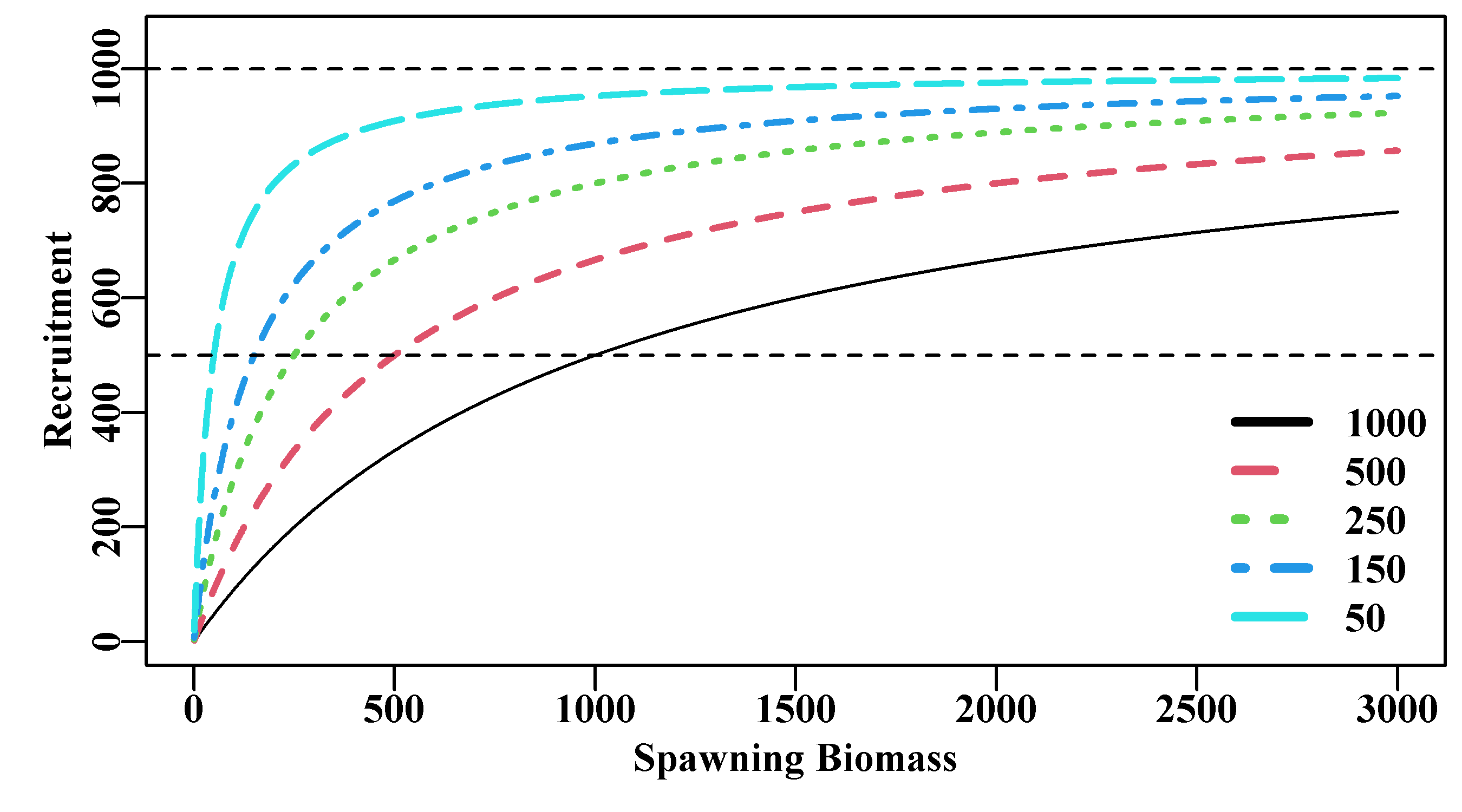
Figure 5.11: The Beverton-Holt stock recruitment curve with a constant a = 1000 and five decreasing b values leading to increasingly productive curves.
5.7.5 Ricker Recruitment
An alternative to the Beverton-Holt curve was suggested by Ricker (1954, 1958), but this also has more than one parameterization:
\[\begin{equation} R_y = a S_y e^{-b{S_y}} e^{\varepsilon} \tag{5.17} \end{equation}\]
where \(R_y\) is the recruitment from \(S_y\), the spawning stock, in year \(y\), \(a\) is the recruits-per-spawner at low stock levels, and \(b\) relates to the rate of decrease of recruits-per-spawner as \(S\) increases. The \(e^{\varepsilon}\) indicates log-normal residual errors between the relationship and observed data. Note well that parameters \(a\) and \(b\) are very different from those in the Beverton–Holt equation. This stock recruitment curve does not attain an asymptote but instead exhibits a decline in recruitment levels at higher stock levels Figure(5.12).
 #plot the MQMF ricker function for Ricker recruitment  Fig 5.12
B <- 1:20000
rickb <- c(0.0002,0.0003,0.0004)
parset()
plot(B,ricker(c(10,rickb[1]),B),type="l",xlab="Spawning Biomass",
               ylab="Recruitment")
for (i in 2:3)
   lines(B,ricker(c(10,rickb[i]),B),lwd=2,col=i,lty=i)
legend("topright",legend=rickb,col=1:3,lty=1:3,bty="n",lwd=2) 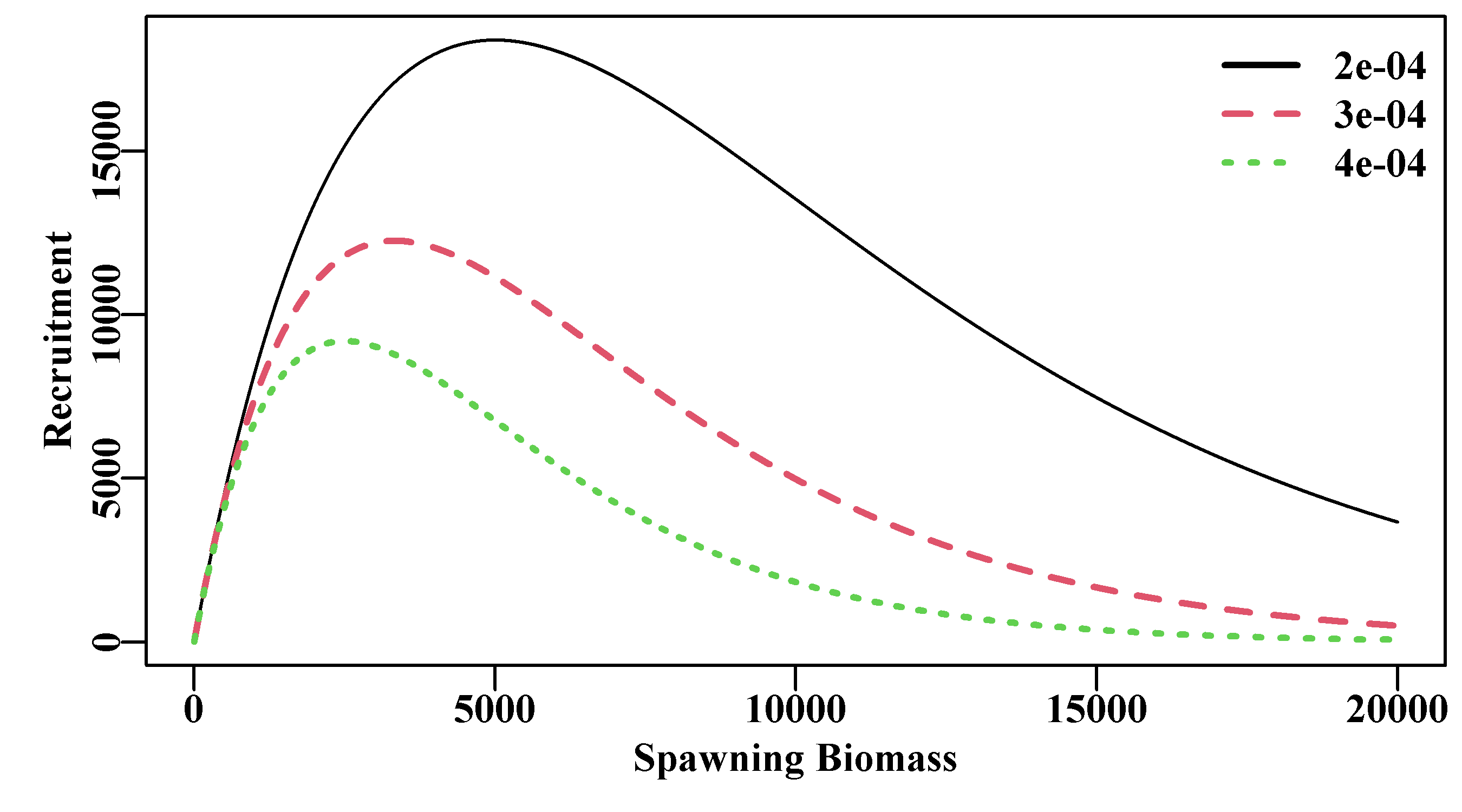
Figure 5.12: Two Ricker stock recruitment curves both with a constant \(a = 10\) but with different \(b\) values. Note that the \(b\) value mainly influences the level of decline in recruitment with increasing biomass and has little effect on the initial steepness.
The idea behind the decline in recruitment with spawning biomass is that it relates to either competitive or predatory effects (cannibalism) of some cohorts on others. Various mechanisms have been proposed including cannibalism of juveniles by adults, density-dependent transmission of disease, damage by spawning adults of each other’s spawning sites (occurs primarily in rivers with fish like salmon), and finally, density-dependent growth combined with size-dependent predation. Each of these mechanisms can lead to different interpretations of the parameters of the Ricker curve.
Once again, the distinction between whether the equation should be interpreted as an explanatory statement about the observable world instead of just a convenient empirical description of the average recruitment becomes important. In addition, while the parameters can certainly be given a real-world interpretation, the equations still tend to be overly simplistic and are best regarded as an empirical description rather than an explanation of events (Punt and Cope, 2019).
5.7.6 Deriso’s Generalized Model
Deriso (1980) proposed a generalized equation for which the Beverton–Holt and the Ricker stock recruitment curves are special cases. Schnute (1985) restructured Deriso’s equation to produce an even more flexible version with even greater flexibility:
\[\begin{equation} {R_y} = \alpha {S_y}(1-\beta \gamma {S_y})^{1/\gamma} \tag{5.18} \end{equation}\]
In this Schnute (1985) generalized case there are three parameters \(\alpha\), \(\beta\), and \(\gamma\), the first two should always be positive but \(\gamma\) can be positive of negative. By modifying the \(\gamma\) value, different special cases arise Figure(5.13):
\[\begin{equation} \begin{split} \gamma =-\infty \;\;\;\; & {{R}_{y}}=\alpha {{B}_{y}} \\ \gamma =-1 \;\;\;\; & {{R}_{y}}=\alpha {{B}_{y}}/(1+\beta {{B}_{y}}) \\ \gamma \to 0 \;\;\;\; & {{R}_{y}}=\alpha {{B}_{y}}{{e}^{-\beta {{B}_{y}}}} \\ \gamma =1 \;\;\;\; & {{R}_{y}}=\alpha {{B}_{y}}(1-\beta {{B}_{y}}) \end{split} \tag{5.19} \end{equation}\]
The arrow in the third case means “approaches”, as in \(\gamma\) approaches zero. The first case is a density-independent constant rate of recruitment, which can also be obtained by setting \(\beta = 0\). The next three cases correspond respectively to the standard stock recruitment relationships of Beverton–Holt (1957), Ricker (1954, 1958), and Schaefer (1954), a form of logistic curve. Of course, in each case care would be required to select appropriate values for \(\alpha\) and \(\beta\).
There are some mathematically unstable properties to the Deriso–Schnute model as should be clear if we were to set \(\gamma = 0\). This would lead to a mathematical singularity (divide by zero). The parameter limits should always be \(\gamma \to 0\), from either the negative or the positive direction. With this equation there are many combinations of parameters that can give rise to implausible stock recruitment relationships. A major value of this equation is demonstrating the relationships between the different curves, one would not use the Deriso-Schnute in a fitted model, though it might be useful in a simulation model.
 # plot of three special cases from Deriso-Schnute curve  Fig. 5.13
deriso <- function(p,B) return(p[1] * B *(1 - p[2]*p[3]*B)^(1/p[3]))
B <- 1:10000
plot1(B,deriso(c(10,0.001,-1),B),lwd=2,
      xlab="Spawning Biomass",ylab="Recruitment")       # BH
lines(B,deriso(c(10,0.0004,0.25),B),lwd=2,col=2,lty=2)  # DS
lines(B,deriso(c(10,0.0004,1e-06),B),lwd=2,col=3,lty=3) # Ricker
lines(B,deriso(c(10,0.0004,0.5),B),lwd=2,col=1,lty=3)   # odd line
legend(x=7000,y=8500,legend=c("BH","DS","Ricker","odd line"),
col=c(1,2,3,1),lty=c(1,2,3,3),bty="n",lwd=3) 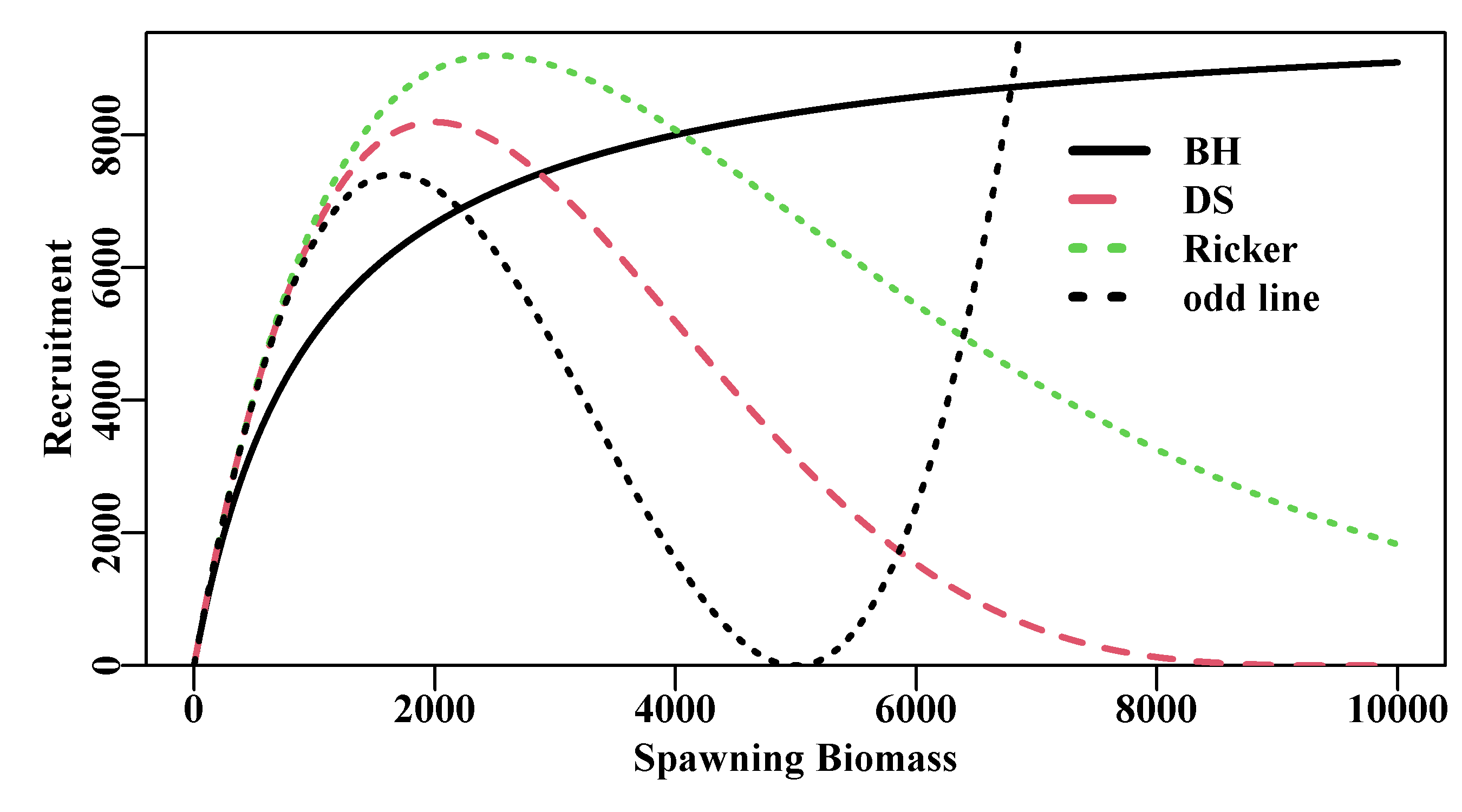
Figure 5.13: A comparison of the Beverton-Holt (BH), Ricker, and Deriso-Schnute (DS) stock recruitment curves, as implemented within the Deriso-Schnute generalized equation Equ(5.19). For the DS curve, a \(\gamma = 0.5\) leads to unrealistic outcomes (odd line).
5.7.7 Re-Parameterized Beverton-Holt Equation
In the chapter Model Parameter Estimation the parameters of a Beverton-Holt stock-recruitment curve were estimated for the tigers data-set concerning tiger prawns. Estimates of relative abundance can equate to recruitment levels in short lived prawn species, but with longer lived species, assessed using age-structured models, estimating such parameters would be relatively abstract. An important development for more complicated stock assessment models was made by Francis (1992) who re-parameterized the Beverton-Holt stock recruitment relationship in terms of the initial steepness of the curve, \(h\), and the initial recruitment, \(R_0\), which was derived from the unfished or virgin spawning biomass \(B_0\). He first used these ideas in what was an age-structured surplus-production model for orange roughy (Haplostethus atlanticus), for which he had catch data, an index of relative abundance from surveys, and biological data relating to growth and weight at age. Using such data he was able to fit the model in a more defensible manner using his more meaningful parameterization of recruitment.
Francis (1992) defined steepness, designated \(h\), as th deterministic number of recruits arising from the stock when the mature biomass is reduced to 20% of its unfished level. He started the description using:
\[\begin{equation} R_0 = \frac{A_0}{\alpha + \beta A_0} \tag{5.20} \end{equation}\]
and thus, by defining steepness, \(h = 0.2B_0\), we obtain:
\[\begin{equation} {h R_0} = \frac{0.2 A_0}{\alpha + \beta 0.2 A_0} \tag{5.21} \end{equation}\]
where \(\alpha\) and \(\beta\) are the Beverton-Holt parameters, \(A_0\) is the total mature biomass per-recruit from the stable age distribution found in an unfished population. The ‘per-recruit’ part is important to age-structured modelling because this permits us to determine a relationship between \(R_0\) and \(B_0\) independently of the Beverton-Holt equation, Equ(5.15). The stable age distribution arises from a constant recruitment level, \(R_0\), exposed to a constant level of natural mortality (\(M\)), leading to a standard exponential decline on numbers-at-age. If natural mortality is low, then a plus group may be needed. That stable age distribution can be defined as:
\[\begin{equation} {{n}_{0,a}}=\left\{ \begin{matrix} {{R}_{0}}{{e}^{-Ma}} & a<{{t}_{\max }} \\ {{R}_{0}}{{e}^{-M{{t}_{\max }}}}/\left( 1-{{e}^{-M}} \right) & a={{t}_{\max }} \\ \end{matrix} \right. \tag{5.22} \end{equation}\]
where \(n_{0,a}\) is the unfished number of fish per-recruit of age \(a\), and \(t_{max}\) is the maximum age being modelled. The \(t_{max}\) acts as a plus group and hence the need for the division by \((1 – {e^{-M}})\), to provide the sum of an exponential series. The biomass \(A_0\) would be the stock biomass that would arise from a constant recruitment level of one. Thus, with a biomass of \(A_0\), distributed across a stable age distribution, the resulting recruitment level would be \(R_0 = 1\) (and vice versa).
\[\begin{equation} {{A}_{0}}=\left( \sum\limits_{m}{{{n}_{0,a}}{{w}_{a}}} \right) \tag{5.23} \end{equation}\]
where \(m\) is the age at maturity, \(n_{0,a}\) is the unfished number of animals per-recruit of age \(a\), and \(w_a\) is the weight of an animal of age \(a\). One can also include part of natural mortality into this equation for it to become equivalent to recruitment part-way through a year. \(A_0\) acts as a scaling factor because a stable age distribution will arise in the unfished population given any constant recruitment level. The magnitude of \(A_0\) will be scaled by the estimated virgin biomass, \(B_0\), but its value, relative to the constant recruitment needed to maintain the stable age distribution, \(R_0\), will remain the same. In practice, one would derive \(A_0\) from biological information and estimate \(R_0\) in the stock assessment model.
\[\begin{equation} {{B}_{0}}= {R_0}\left( \sum\limits_{m}{{{n}_{0,a}}{{w}_{a}}} \right) = \left( {R_0}{A_0} \right) \tag{5.24} \end{equation}\]
Francis (1992) then also used his definition of recruitment steepness to re-parameterize the Beverton-Holt parameters \(a\), \(b\), \(\alpha\), and \(\beta\) (see Appendix to this chapter):
\[\begin{equation} {a} = \frac{4h{R_0}}{(5h-1)} \;\;\;\; {b} = \frac{{B_0}(1-h)}{(5h-1)} \tag{5.25} \end{equation}\]
Substituting these into Equ(5.16) we obtain:
\[\begin{equation} {R_y} = \frac{{\frac{4hR_0}{(5h-1)}{B_y}}}{\frac{{B_0}(1-h)}{(5h-1)}+{B_y}} \tag{5.26} \end{equation}\]
Dropping the upper level \((5h-1)\) to the lower level:
\[\begin{equation} {R_y} = \frac{{{4hR_0}{B_y}}}{\frac{(5h-1){B_0}(1-h)}{(5h-1)}+(5h-1){B_y}} \tag{5.27} \end{equation}\]
then cancelling out the \((5h-1)\) where possible leaves the Beverton-Holt redefined in terms of steepness \(h\), \(B_0\) and \(R_0\), which all have more meaningful interpretations and using Equ(5.25), or Equ(5.28), would be more easily estimable in an assessment model:
\[\begin{equation} R_y = \frac{4hR_0 B_y}{B_0(1-h)+B_y(5h-1)} \tag{5.28} \end{equation}\]
5.7.8 Re-Parameterized Ricker Equation
In a similar fashion, The Ricker stock recruitment equation can be re-parameterized in terms of steepness \(h\), \(B_0\) and \(R_0\):
\[\begin{equation} R_y = \frac{{R_0}{B_y}}{B_0} exp{\left( h \left(1-\frac{B_y}{B_0} \right)\right)} \tag{5.29} \end{equation}\]
Both Equs(5.25) and (5.28) are now the more commonly used parameterizations used in stock assessments and simulation models that attempt to include recruitment.
5.8 Selectivity
5.8.1 Introduction
Another class of static models used within stock assessment models (and simulations) relate to the selectivity of fishing gear for particular species. The idea being that if a population of an exploited species is available in an area then if a particular fishing gear is used (a trawl, a Danish seine, a gill-net, a lobster pot, etc) then the construction of the gear and how it is used will influence which members of the available population will be vulnerable to the gear if they encounter it. The notion of selectivity within, say, an age-structured assessment model is complicated by the notion of availability. If, for example, the main fishing grounds for a species are in waters deeper than 250 m and predominantly only smaller juveniles are present in shallower waters then if one were to estimate the selectivity of the gear using data only from the shallower water one would likely get a different answer from an estimate made with data from deeper waters. In fact, selectivity curves estimated within assessment models should really be regarded as selectivity/availability curves.
The choice of the shape of a selectivity curve is an important decision. Some fishing gears typically have selectivity described by specific equations. Thus, the selectivity of trawl gears are often described using a logistic equation, whereas long-line gear (using hooks) is often described using a dome shaped selectivity function.
One can only fit such models of selectivity within stock assessment models if there are age- or size-composition data available from the catches. As we saw in the Model Parameter Estimation chapter, one would usually fit such composition data using multinomial likelihoods. Within a stock assessment model one would normally model the stock dynamics in terms of expected numbers-at-age, which would imply certain numbers-at-size. So, when attempting to generate predicted catch composition data (of either ages or sizes) one needs to multiply the available numbers-at-age or size by the predicted selectivity. Thus, during the fitting process the composition data contribute to the estimation of the selectivity parameters.
Here we will merely illustrate alternative selectivity equations and show their different properties.
5.8.2 Logistic Selection
There are many different equations used to describe the selectivity characteristics of different fishing gears but an extremely common one is the standard logistic or S-shaped curve, which is typical for trawl gear selectivity. It implies that the vulnerability to the gear will gradually increase as age or size increases until 100% are vulnerable if they encounter the gear (this gradual increase to 100% is the same as we saw in maturity). Two equations are commonly used, the first is described by the MQMF function logist():
\[\begin{equation} {s_a}=\frac{1}{1+{{e}^{-\log{(19)}{(a-{a_{50}})}/{\delta }}}} \tag{5.30} \end{equation}\]
where \(s_a\) is the selectivity-at-age (a proportion) for age \(a\), \(a_{50}\) is the age at which 50% selectivity occurs, and \(\delta\) is the gradient of the curve defined as the number of years from a selectivity of 50% to a selectivity of 95%. Where we talk of age we could equally be talking of size. The upper bound of \(\delta\) as 95% (\(\delta\) is actually \(L95 - L50\)). An alternative logistic curve, that we have already seen in the section Selectivity in YPR within the Simple Population Models chapter, and was also used to describe maturity-at-age, is defined in the function mature():
\[\begin{equation} {{s}_{a}}=\frac{1}{1+{{({{e}^{(\alpha +\beta a)}})}^{-1}}}=\frac{{{e}^{(\alpha +\beta a)}}}{1+{{e}^{(\alpha +\beta a)}}} \tag{5.31} \end{equation}\]
where \(\alpha\) and \(\beta\) are the logistic parameters, and \(-\alpha/\beta\) is the age at a selectivity of 0.5 (50%). The inter-quartile distance (literally quantile 25% to quantile 75%) is defined as \(IQ = 2 \log{(3)} /\beta\) (see the MQMF function mature() for an implementation of this function). Generally, in age-structured modelling one needs length- or age-composition data so that the gear selectivity combined with fishery availability can be estimated directly. When working with yield-per-recruit calculations the usual reason to include a form of selectivity is to determine the optimum age at which to begin applying fishing mortality. For this reason what is known as knife-edged selectivity is often used, which essentially identifies the specific age below which there is no selection and above which there is 100% selection. This is implemented in the MQMF function logist(); knife-edged selectivity no longer tends to be used in full age-structured stock assessment models, although it is still used in delay-difference models (Schnute, 1985; Hilborn and Walters, 1992).
 #Selectivity curves from logist and mature functions  See Fig 5.14
ages <- seq(0,50,1);   in50 <- 25.0
sel1 <- logist(in50,12,ages)         #-3.65/0.146=L50=25.0
sel2 <- mature(-3.650425,0.146017,sizeage=ages)
sel3 <- mature(-6,0.2,ages)
sel4 <- logist(22.0,14,ages,knifeedge = TRUE)
plot1(ages,sel1,xlab="Age Years",ylab="Selectivity",cex=0.75,lwd=2)
lines(ages,sel2,col=2,lwd=2,lty=2)
lines(ages,sel3,col=3,lwd=2,lty=3)
lines(ages,sel4,col=4,lwd=2,lty=4)
abline(v=in50,col=1,lty=2); abline(h=0.5,col=1,lty=2)
legend("topleft",c("25_eq5.30","25_eq5.31","30_eq5.31","22_eq5.30N"),
col=c(1,2,3,4),lwd=3,cex=1.1,bty="n",lty=c(1:4)) 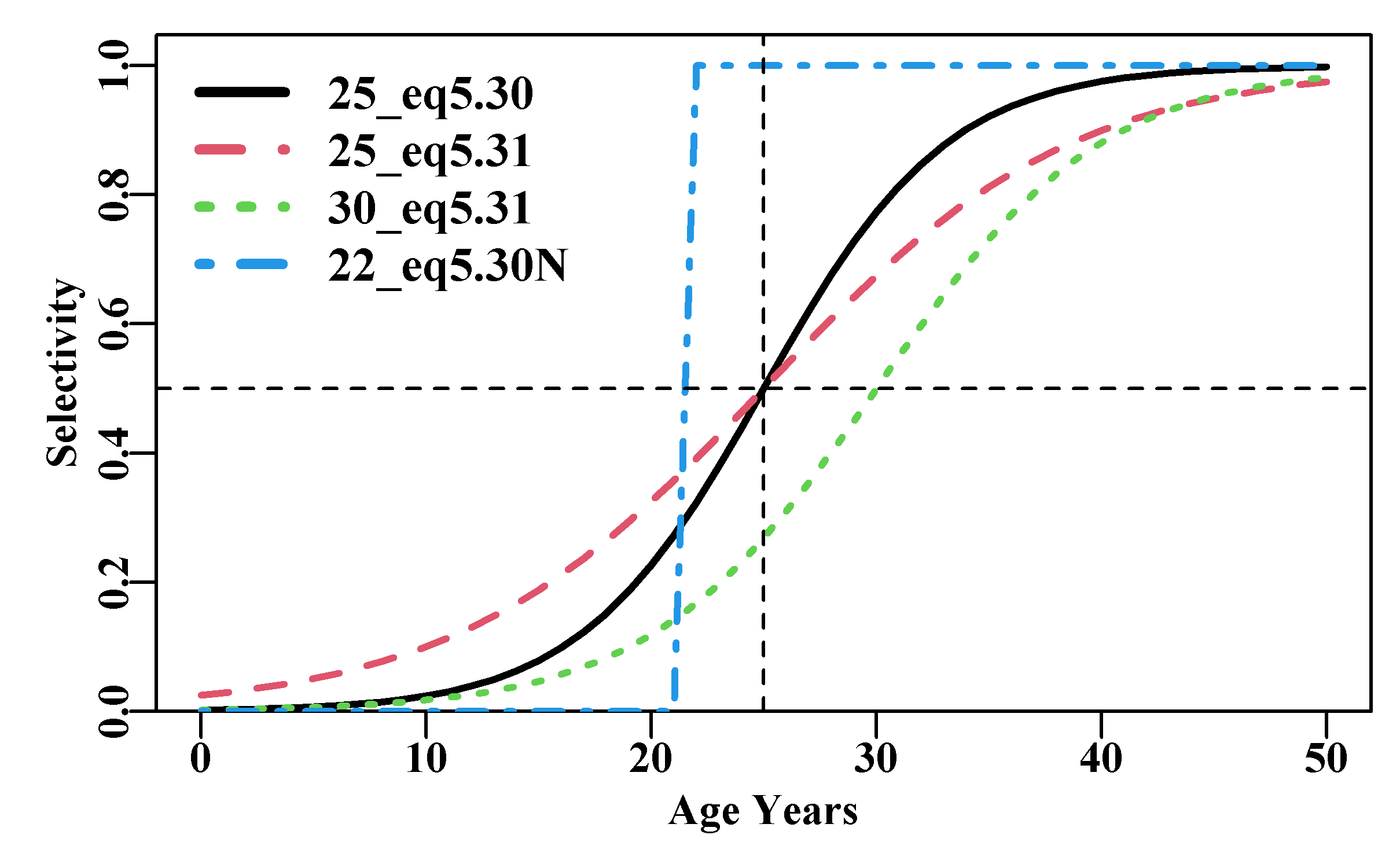
Figure 5.14: Examples of the logistic S-shaped curve from the logist() and mature() functions. The dashed red and solid black curves have the same L50, though different gradients. The dotted green illustrate the effect of varying the b parameter of the mature() function, while the hashed blue curve illustrates knife-edged selection. The legend depicts the L50 and the equation used.
5.8.3 Dome Shaped Selection
A selectivity pattern that ascends to a peak, may possibly have a plateau, and then has a descending limb is termed dome-shaped and is typical of fishing gear such as gill-nets and hook based gear such as long-lines. Having so many components such selectivity curves tend to be much more complex because the ascending, plateau, and descending parts all need to be joined together. Modern approaches to fitting such models tend to use auto-differentiation software such as AD-Model Builder or related software (Bull et al, 2012; Fournier et al, 2012; Kristensen et al, 2016). This means component models within an assessment model need to be differentiable so the joints between the three components of a domed selectivity curve need to be continuous (Methot and Wetzell, 2013; Hurtado-Ferro et al, 2014). Such an equation would have at least five components the ascending limb, \(asc\), the flat top where selectivity equals 1.0, the descending limb, \(dsc\), and two joining functions, \(J_1\) and \(J_2\), between between the primary three, Equ(5.32):
\[\begin{equation} {{s}_{L}}=asc\left( 1-{{J}_{1,L}} \right)+{{J}_{1,L}}\left( \left( 1-{{J}_{2,L}} \right)+{{J}_{2,L}}dsc \right) \tag{5.32} \end{equation}\]
where \(s_L\) is the selectivity of length \(L\). The various component functions are defined as:
\[\begin{equation} \begin{split} & asc=1-\left( 1-{{\lambda }_{5}} \right)\left( \frac{1-\exp \left( {{\left( {{m}_{L}}-{{\lambda }_{1}} \right)}^{2}}/{{\lambda }_{3}} \right)}{1-\exp \left( {{\left( {{m}_{\min }}-{{\lambda }_{1}} \right)}^{2}}/{{\lambda }_{3}} \right)} \right) \\ & dsc=1-\exp \left( -\left( {{\left( {{m}_{L}}-{{\lambda }_{2}} \right)}^{2}}/{{\lambda }_{4}} \right) \right) \\ & {{J}_{1,L}}=1/\left( 1+\exp \left( -\left( {{m}_{L}}-{{\lambda }_{1}} \right)/\left( 1+\left| {{m}_{L}}+{{\lambda }_{1}} \right| \right) \right) \right) \\ & {{J}_{2,L}}=1/\left( 1+\exp \left( -\left( {{m}_{L}}-{{\lambda }_{2}} \right)/\left( 1+\left| {{m}_{L}}+{{\lambda }_{2}} \right| \right) \right) \right) \end{split} \tag{5.33} \end{equation}\]
where \(m_L\) is the mean length of length class \(L\), \(m_{min}\) is the mean size of the smallest length class, \(\lambda_1\) is the size at which selectivity reaches 1.0, \(\lambda_2\) is the size at which selectivity starts decreasing from 1.0 (if \(\lambda_1\) and \(\lambda_2\) are equal there would be no plateau), \(\lambda_3\) affects the slope of the ascending limb, \(asc\), \(\lambda_4\) affects the slope of the descending limb, \(dsc\), \(\lambda_5\) is the log of the selectivity at \(m_{min}\), and \(\lambda_6\) is the log of the selectivity of the \(m_{max}\), Figure(5.15).
There are thus six parameters \(\lambda_1\) to \(\lambda_6\) required, along with the mean lengths of the length classes used, to define this domed selectivity curve.
 #Examples of domed-shaped selectivity curves from domed. Fig.5.15
L <- seq(1,30,1)
p <- c(10,11,16,33,-5,-2)
plot1(L,domed(p,L),type="l",lwd=2,ylab="Selectivity",xlab="Age Years")
p1 <- c(8,12,16,33,-5,-1)
lines(L,domed(p1,L),lwd=2,col=2,lty=2)
p2 <- c(9,10,16,33,-5,-4)
lines(L,domed(p2,L),lwd=2,col=4,lty=4) 
Figure 5.15: Three examples of domed-shaped selectivity curves produced by the function domed(), with changes to the initial age at achieving a selectivity of 1.0 (10, 8, 9), and the age (11, 12, 10) at which that stops, as well as the selectivity of the final age class.
5.9 Concluding Remarks for Static Models
Stock assessment models that are more complex than the surplus production models we have considered are mostly combinations of dynamic models of the progression of cohorts mixed up with a collection of static models of the kind illustrated in this chapter. Thus, a knowledge of models of growth, maturity, selectivity and recruitment is essential for any understanding of the structure of more advanced models. Sometimes one would estimate their parameters outside of an assessment model but often the estimation would be part of fitting the whole stock assessment model. The advantage of fitting all the separate model components at once is that any interctions between the components can be automatically accounted for.
This chapter has provided an introductory foundation to quite an array of static models. The objective being that if and when you come across alternatives you will be able to use them and fit them in a manner similar to the methods we have used here. Each such models have their own set of assumptions. As long as you are aware of those assumptions you should be able to defend decisions you make concerning which static models to use in your own modelling.
5.10 Appendix: Derivation of Fabens Transformation
Fabens (1965) transformed the von Bertalanffy growth curve so that it matched the data made available from tagging programmes (the length and date at tagging, and the length and date at recapture). The length-at-age version of the von Bertalanffy curve is:
\[\begin{equation} \hat{L}_{t}={L}_{\infty }\left( 1-{{e}^{\left( -K\left( t-{{t}_{0}} \right) \right)}} \right) + N(0,\sigma) \tag{5.34} \end{equation}\]
which, in a tagging context has a length after a given time increment (\(\Delta t\)) defined thus:
\[\begin{equation} {{L}_{t+\Delta t}}={{L}_{\infty }}-{{L}_{\infty }}{{e}^{-K\left( \left( t+\Delta t \right)-{{t}_{0}} \right)}} \tag{5.35} \end{equation}\]
Being in the exponential term the contribution from the \(\Delta t\) can be extracted:
\[\begin{equation} {{L}_{t+\Delta t}}={{L}_{\infty }}-{{L}_{\infty }}{{e}^{-K\left( t-{{t}_{0}} \right)}}{{e}^{-K\Delta t}} \tag{5.36} \end{equation}\]
Now the growth increment \(\Delta L\) expected to occur during \(\Delta t\) can be defined as \(L_t\) subtracted from \(L_{t + \Delta t}\):
\[\begin{equation} \begin{split} & \Delta {L}=\left( {{L}_{t+\Delta t}}-{{L}_{t}} \right)= \\ & \left( {{L}_{\infty }}-{{L}_{\infty }}{{e}^{-K\left( t-{{t}_{0}} \right)}}{{e}^{-K\Delta t}} \right)-\left( {{L}_{\infty }}-{{L}_{\infty }}{{e}^{\left( -K\left( t-{{t}_{0}} \right) \right)}} \right) \end{split} \tag{5.37} \end{equation}\]
We can remove the brackets, which will alter the negation in the second term to a plus and then re-arrange the separated terms.
\[\begin{equation} \Delta {L}={{L}_{\infty }}-{{L}_{\infty }}{{e}^{-K\left( t-{{t}_{0}} \right)}}{{e}^{-K\Delta t}}-{{L}_{\infty }}+{{L}_{\infty }}{{e}^{\left( -K\left( t-{{t}_{0}} \right) \right)}} \tag{5.38} \end{equation}\]
The two isolated \(L_{\infty}\) terms can be cancelled out to improve the clarity of the demonstration, but they will be returned a little later. In addition we can re-arrange the two remaining exponential terms:
\[\begin{equation} \Delta {L}={{L}_{\infty }}{{e}^{\left( -K\left( t-{{t}_{0}} \right) \right)}}-{{L}_{\infty }}{{e}^{-K\left( t-{{t}_{0}} \right)}}{{e}^{-K\Delta t}} \tag{5.39} \end{equation}\]
the re-arrangement makes it possible to extract out a \({L}_{\infty }e^{\left( -K\left( t-{{t}_{0}} \right) \right)}\) term to simplify the whole:
\[\begin{equation} \Delta {L}={{L}_{\infty }}{{e}^{\left( -K\left( t-{{t}_{0}} \right) \right)}}\left( 1-{{e}^{-K\Delta t}} \right) \tag{5.40} \end{equation}\]
So now we can shift the \(\Delta t\) term to the left and return the \(L_{\infty} - L_{\infty}\) term:
\[\begin{equation} \frac{\Delta L}{\left( 1-{{e}^{-K\Delta t}} \right)}={{L}_{\infty }}-{{L}_{\infty }}+{{L}_{\infty }}{{e}^{\left( -K\left( t-{{t}_{0}} \right) \right)}} \tag{5.41} \end{equation}\]
If we add some brackets, which will reverse the plus to a minus, we can finally reach the point of recognizing the combination of terms that equals \(L_t\):
\[\begin{equation} \frac{\Delta \hat{L}}{\left( 1-{{e}^{-K\Delta t}} \right)}={L_{\infty }}-\left( {L_{\infty }}-{{L}_{\infty }}{{e}^{\left( -K\left( t-{t_0} \right) \right)}} \right)=\left( {L_{\infty } }-{L_t} \right) \tag{5.42} \end{equation}\]
which, by returning the \(\Delta t\) term to the right results in the classical Fabens growth increment equation:
\[\begin{equation} \Delta L=\left( {L_{\infty }}-{L_t} \right)\left( 1-{e^{-K\Delta t}} \right) \tag{5.43} \end{equation}\]
It is important to note that this transformation also transforms the Normal random residuals from the length-at-age equation, which, of course, are used when estimating the parameters. This implies the parameters, even though they have the same names, are not strictly comparable.
5.11 Appendix: Reparameterization of Beverton-Holt
Francis (1992) provides definitions of the Beverton–Holt parameters in terms of the more biologically meaningful terms relating to steepness (\(h\)), virgin mature biomass (\(B_0\)), and virgin recruitment (\(R_0\)). Rather than use
\[\begin{equation} R_y = \frac{B_{y-1}}{\alpha + \beta B_{y-1}} \tag{5.44} \end{equation}\]
the alternative formulation is used, although, at the end, we will revert to using the relationships \(\alpha = b/a\) and \(\beta = 1/a\).
Thus we will use:
\[\begin{equation} R_y = \frac{aB_y}{b + B_y} \tag{5.45} \end{equation}\]
where \(R_y\) is the recruitment in year \(y\), \(B_y\) is the spawning stock size in year \(y\), and \(a\) and \(b\) are the Beverton–Holt parameters. In an unfished equilibrium state we can couch the equation as:
\[\begin{equation} R_0 = \frac{aB_{0}}{b + B_{0}} \tag{5.46} \end{equation}\]
Steepness (\(h\)) is defined as the recruitment obtained at 20% of virgin biomass:
\[\begin{equation} hR_0 = \frac{0.2aB_{0}}{b + 0.2B_{0}} \tag{5.47} \end{equation}\]
If the equilibrium equation for \(R_0\) is substituted into this equation we obtain:
\[\begin{equation} h \frac{aB_{0}}{b + B_{0}}=\frac{0.2aB_{0}}{b + 0.2B_{0}} \tag{5.48} \end{equation}\]
and hence:
\[\begin{equation} h = \frac{\left(0.2aB_0 \right) \left(b +B_0 \right)}{ \left( b + 0.2B_0 \right) \left(aB_0 \right )}=\frac{0.2\left(b+B_0 \right)}{b+0.2B_0} \tag{5.49} \end{equation}\]
Multiplying through leads to:
\[\begin{equation} hb +0.2hB_0 = 0.2b+ 0.2B_0 \tag{5.50} \end{equation}\]
and exchanging terms to isolate \(b\) and \(B_0\) and multiplying by 5 to remove the 0.2 values:
\[\begin{equation} 5hb - b = B_0 - hB_0 \tag{5.51} \end{equation}\]
and simplifying leads to:
\[\begin{equation} b \left(5h - 1\right)=B_0 \left(1-h \right) \tag{5.52} \end{equation}\]
thus \(b\) can be reparameterized as:
\[\begin{equation} b = \frac{B_0 \left(1-h \right)}{\left(5h - 1\right)} \tag{5.53} \end{equation}\]
This version of \(b\) can be used in our original equation and re-arranged to do something similar for the \(a\) parameter:
\[\begin{equation} R_0 = \frac{aB_0}{\frac{B_0 \left(1-h \right)}{\left(5h - 1\right)}+ B_0} \tag{5.54} \end{equation}\]
which converts to:
\[\begin{equation} R_0 \frac{B_0 \left(1-h \right)}{\left(5h - 1\right)} + R_0 B_0 = aB_0 \tag{5.55} \end{equation}\]
Dividing through by \(B_0\) and then multiplying the second \(R_0\) on the left hand of the \(=\) by \(5h – 1\) allows a simplification:
\[\begin{equation} \frac{R_0- hR_0 + 5hR_0 - R_0}{5h -1} = \frac{4hR_0}{5h-1} = a \tag{5.56} \end{equation}\]
Remember that \(\alpha = b/a\) and \(\beta = 1/a\), so we can finish with
\[\begin{equation} \alpha = b \times 1/a = \frac{B_0 \left(1-h \right)}{\left(5h - 1\right)} \times \frac{5h-1}{4hR_0} = \frac{B_0 (1-h)}{4hR_0} \tag{5.57} \end{equation}\]
and
\[\begin{equation}
\beta = 1/a = \frac{5h-1}{4hR_0}
\tag{5.58}
\end{equation}\]
as defined by Francis (1992). This has redefined the Beverton- Holt model parameters in terms of \(h\), \(B_0\), and \(R_0\). The relationship required between \(B_0\) and \(R_0\) is required but we cannot use the equilibrium equation for that so instead we assume that the unfished population is in equilibrium with a stable age distribution. The mature biomass generated per recruit from the stable age distribution (\(A_0\)) therefore defines the required relationship between \(B_0\) and \(R_0\).