Chapter 3 Simple Population Models
3.1 Introduction
Simple population models form the foundations of numerous fisheries models, indeed the separation of fisheries modelling from ecological population modelling is only an artificial distinction. Understanding how any population model operates should be useful for an improved understanding of fisheries models and so in this chapter we are going to use R to examine the dynamics of some of the fundamental ideas in population biology.
3.1.1 The Discrete Logistic Model
We will first examine the dynamics exhibited by what has become one of the classical population models in ecology, the discrete logistic model. This model crops up in very many places and in many different forms and is thus worth exploring in some detail. Here we will use the Schaefer (1954, 1957) version, which has four components or terms:
\[\begin{equation} \begin{split} {N_{t=0}} &= N_0 \\ {{N}_{t+1}} &= {{N}_{t}}+{{r}{N}_{t}}\left( 1-{{\left( \frac{{{N}_{t}}}{K} \right)}} \right)-{{C}_{t}} \end{split} \tag{3.1} \end{equation}\]
The term, \(N_t\), is the numbers-at-time \(t\) (e.g. at the start of year \(t\)), and the last term is \(C_t\), which is the catch in numbers taken in time \(t\) (e.g. during the year \(t\)). The first line reflects the initial conditions, defined as the numbers (or biomass) at time zero. Be wary of the sub-scripts as, with either numbers or biomass, they refer to particular times, usually the start of the identified time period \(t\), whereas with catches they refer to the catches taken throughout the time period \(t\). The equation is a summary of the dynamics across the time-step \(t\); it is a difference equation not a continuous differential equation. The middle term of the second equation is a more complex component that defines what is termed the production curve in fisheries. This is made up of \(r\), which is known as the intrinsic rate of population growth and \(K\), which is the carrying capacity or maximum population size. If the dynamics are represented as being before exploitation began and at equilibrium then the \(N_0\) would take the same value as \(K\), but it is kept separate to allow for deviations from equilibrium at the beginning of any time-series. In the MQMF discretelogistic() function you will see another parameter, p, which will be examined in detail in the chapter on Surplus Production Models. It suffices here to state that with the default value of \(p = 1.0\) the equation is equivalent to the Schaefer model in Equ(3.1). Here, the Schaefer model is written out using numbers-at-time although in fisheries it is commonly used directly with biomass-at-time (\(B_t\)). The fact that these terms can be altered in this way emphasizes that this model ignores biological facts and properties such as size- and age-structure within a population, as well as any differences between the sexes and other properties. The surprising thing is that such a simple model can still be as useful as it is in both theory and practice.
We can illustrate the production curve by plotting the central term from Equ(3.1) against a vector of \(N_t\) values. The sub-term \(rN_{t}\) represents unconstrained exponential population growth and this term is added to \(N_t\) in this discrete form of the equation. Thus, as long as \(r > 0.0\) and catches are zero, we would expect un-ending positive population growth from the \({{N}_{t}}+{{r}{N}_{t}}\) part of the equation. However, the sub-term \((1-(Nt/K))\) acts to constrain the exponential growth term and does so more and more as the population size increases. This acts as, and is known as, a density-dependent effect.
 #Code to produce Figure 3.1. Note the two one-line functions
surprod <- function(Nt,r,K) return((r*Nt)*(1-(Nt/K)))
densdep <- function(Nt,K) return((1-(Nt/K)))
r <- 1.2; K <- 1000.0; Nt <- seq(10,1000,10)
par(mfrow=c(2,1),mai=c(0.4,0.4,0.05,0.05),oma=c(0.0,0,0.0,0.0))
par(cex=0.75, mgp=c(1.35,0.35,0), font.axis=7,font=7,font.lab=7)
plot1(Nt,surprod(Nt,r,K),xlab="Population Nt",defpar=FALSE,
      ylab="Production")
plot1(Nt,densdep(Nt,K),xlab="Population Nt",defpar=FALSE,
ylab="Density-Dependence") 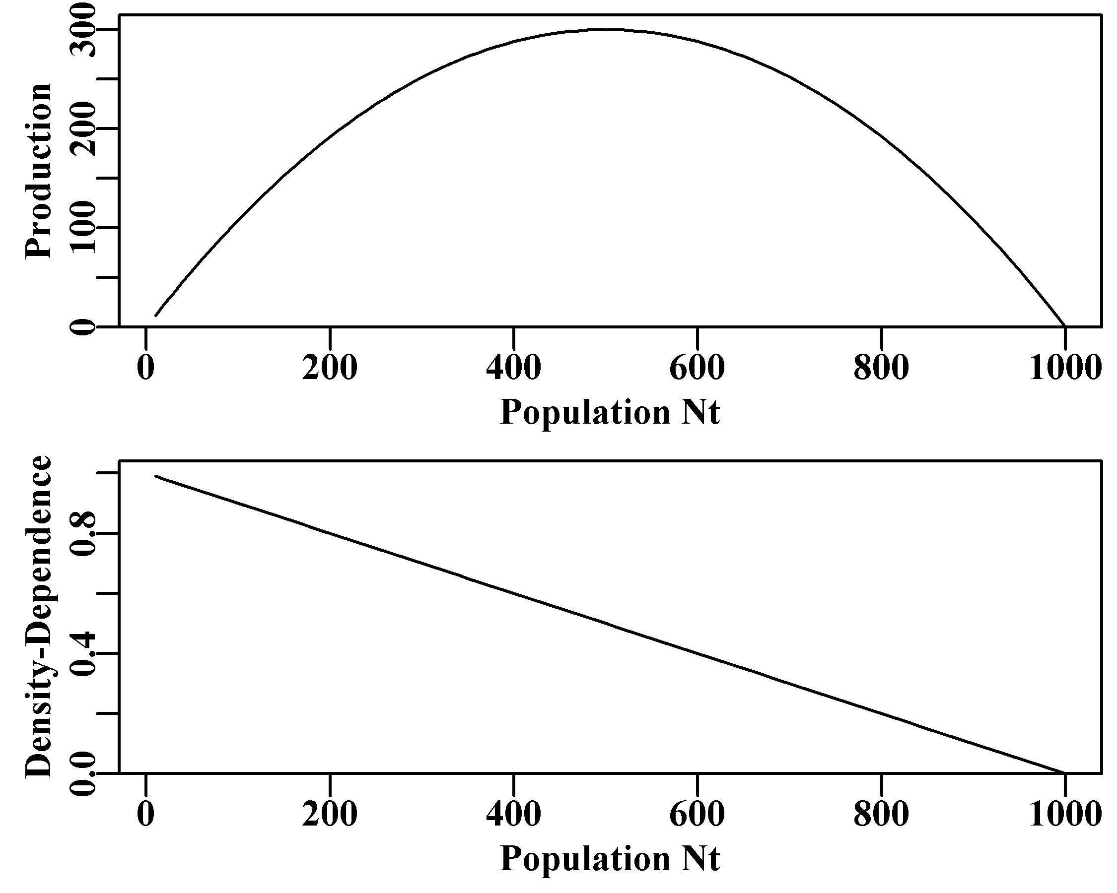
Figure 3.1: The full production curve for the discrete Schaefer (1954, 1957) surplus production model and the equivalent implied linear density dependent relationship with population size.
Density-dependence is an important part of population size regulation (May and McLean, 2007). As is apparent in Figure(3.1), the density-dependent term in the Schaefer model has a descending linear relationship with population size. This is literally what is meant by the phrase “linear density-dependence”, which you will find in the population dynamics literature. This density-dependent term, attempts to compensate for the exponential increases driven by the \(rN_t\) term and constrain the population size to no larger than the long-term average unfished population size \(K\) (see the next section for what happens when that compensation is insufficient).
3.1.2 Dynamic Behaviour
The differential equation version of the Schaefer model was always known as being very stable with the maximum population size truly being constrained to the \(K\) value. It was with some surprise that the dynamics of the discrete version were found to be much more complex and interesting (May, 1973, 1976). We have implemented a version of the equation above in the function discretelogistic() whose help file you can read via ?discretelogistic and whose code can be seen by entering discretelogistic into the console (note no brackets). If you examine the code in this function you will see that it uses a for loop to step through the years to calculate the population size each year. Hopefully, as an R programmer, you will be wondering why I did not use a vectorized approach to avoid the use of the for loop. This highlights a fundamental aspect of population dynamics, the numbers at time \(t\) are invariably a function of the numbers at time \(t - 1\) (initial conditions can differ from this, hence the \(N_0\) parameter). The sequential nature of population dynamics means that we cannot use vectorization in any efficient manner. The sequential nature of population dynamics is such an obvious fact that the constraints and structure that it imposes on population models often go unnoticed.
The discretelogistic() function outputs (invisibly) a matrix of the time passed, \(year\) (as year), the numbers at time \(t\), \(n_t\) (as nt), and the numbers at time \(t+1\), \(n_{t+1}\) (as nt1). This matrix is also given the class dynpop and a plot S3 method is included in MQMF (plot.dynpop; see A non-introduction to R for the use of S3 classes and methods. To see the code type MQMF:::plot.dynpop into the console, note the use of three colons not two). The S3 method is used to produce a standardized plot of the outcome from discretelogistic(), though, of course, one could write any alternative one wanted. Try running the code below sequentially with the values of rv set to 0.5, 1.95, 2.2, 2.475, 2.56, and 2.8.
 #Code for Figure 3.2. Try varying the value of rv from 0.5-2.8
yrs <- 100; rv=2.8;  Kv <- 1000.0; Nz=100; catch=0.0; p=1.0
ans <- discretelogistic(r=rv,K=Kv,N0=Nz,Ct=catch,Yrs=yrs,p=p)
avcatch <- mean(ans[(yrs-50):yrs,"nt"],na.rm=TRUE) #used in text
label <- paste0("r=",rv," K=",Kv," Ct=",catch, " N0=",Nz," p=",p=p)
plot(ans, main=label, cex=0.9, font=7) #Schaefer dynamics 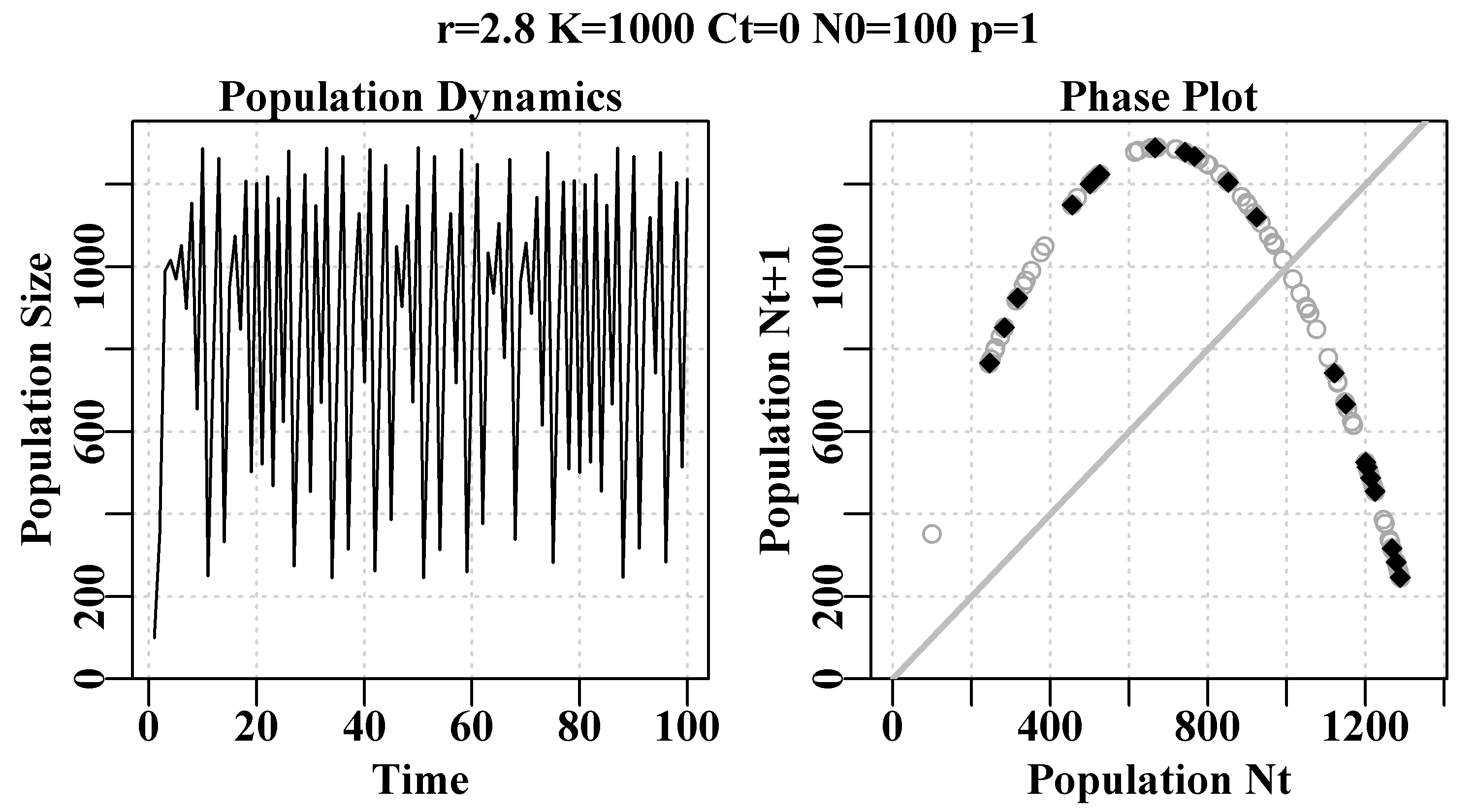
Figure 3.2: Schaefer model dynamics. The left plot is the numbers by year, illustrating chaotic dynamics from an r-value of 2.8. The right plot is numbers-at-time t+1 against time t, known as a phase plot. The final 20% of points are in red to illustrate any equilibrium behaviour. The grey diagonal is the 1:1 line.
If you ran the code that gives rise to Figure(3.2), with the six values of rv mentioned above, you should have seen a monotonically damped equilibrium (one solid dot), then a damped oscillatory equilibrium (still one solid dot), then something between a damped oscillatory equilibrium and a 2-cycle stable limit cycle (somewhat smeared two solid dots). With r = 2.475 there is a 4-cycle stable limit cycle (4 solid dots), and with r = 2.56 an 8-cycle stable limit cycle. Finally, with r = 2.8 the dynamics end in chaos in which the outcome at each step is not random but neither is it directly predictable, although all points fall on the parabola that can be seen in the right-hand plot. In Chaos theory this parabola is known as a strange attractor, although this is a very simple one. Such chaotic systems are also dependent on the starting conditions. If you change the initial numbers to 101 instead of 100 the time-line of numbers changes radically, although the parabola remains the same. Of course one can input any range of numbers desired, one could also alter the dynamics by using a slightly different model. While chaos is interesting and fun to play with (Gleick, 1988; Lauwerier, 1991) it seems to be rarely useful in real world applications of modelling natural populations. Indeed, some have claimed that the apparent randomness in their observations was brought about by population responses to stochastic environmental effects rather than by the non-linearity introduced by under- and over-compensation in a density-dependent model (Higgins et al, 1997).
In practical terms, if you were to find a model was giving rise to apparently chaotic or cyclic behaviour, or even negative population numbers, it would be sensible to try to determine whether what was being observed was real biological population behaviour (obviously not the negative numbers) or, more simply, just a mathematical expression of unusual parameters. One could always force avoidance of a model dropping below \(0\) by including something like \(max((B_t + (rB_t)(1-(B_t/K)) - C_t),0)\) in the calculation (see the discretelogistic() code. Analogously, Values far above \(K\) could be avoided by \(min((B_t + (rB_t)(1-(B_t/K)) - C_t),1.1K)\), although such additions to the code remain ad hoc (should, for example, any over-shoot above \(K\) be allowed, as in \(1.1K\), or should it be \(1.0K\)?; some populations are naturally variable). In Surplus Production Models we will examine the use of penalty functions that can be used to prevent anomalous values arising when estimating such parameters while avoiding the use of blunt instruments such as max(...,0).
We can examine the actual population size each year by directing the invisible output from the discretelogistic() function into an object which can then be worked with, Table(3.1).
 #run discrete logistic dynamics for 600 years
yrs=600
ans <- discretelogistic(r=2.55,K=1000.0,N0=100,Ct=0.0,Yrs=yrs)
When we set the r value to generate a 2-cycle stable limit (e.g. \(r = 2.2\)) this can be clearly seen in the repetition of the numbers in alternative years. Examining the actual numbers-at-time is clearly more accurate than trusting to a visual impression from a plot. This also means we can interrogate the outcome in as much detail as we wish. In the case above the mean of the last 50 years of catches was 859.675, which is obviously less than the K of 1000. Because of the phase relationship Nt+1 vs Nt the final line in the last year would not normally have an Nt+1 value, so, in the code the number of years input is incremented by one so that a final \(N_{t+1}\) is generated (see the code).
| year | nt | nt1 | year | nt | nt1 | year | nt | nt1 |
|---|---|---|---|---|---|---|---|---|
| 571 | 493.9 | 1131.3 | 581 | 752.4 | 1227.4 | 591 | 515.6 | 1152.4 |
| 572 | 1131.3 | 752.4 | 582 | 1227.4 | 515.6 | 592 | 1152.4 | 704.5 |
| 573 | 752.4 | 1227.4 | 583 | 515.6 | 1152.4 | 593 | 704.5 | 1235.4 |
| 574 | 1227.4 | 515.6 | 584 | 1152.4 | 704.5 | 594 | 1235.4 | 493.9 |
| 575 | 515.6 | 1152.4 | 585 | 704.5 | 1235.4 | 595 | 493.9 | 1131.3 |
| 576 | 1152.4 | 704.5 | 586 | 1235.4 | 493.9 | 596 | 1131.3 | 752.4 |
| 577 | 704.5 | 1235.4 | 587 | 493.9 | 1131.3 | 597 | 752.4 | 1227.4 |
| 578 | 1235.4 | 493.9 | 588 | 1131.3 | 752.4 | 598 | 1227.4 | 515.6 |
| 579 | 493.9 | 1131.3 | 589 | 752.4 | 1227.4 | 599 | 515.6 | 1152.4 |
| 580 | 1131.3 | 752.4 | 590 | 1227.4 | 515.6 | 600 | 1152.4 | 704.5 |
3.1.3 Finding Boundaries between Behaviours.
One can find when a stable limit cycle arises by averaging the rows of the \(nt\) and \(nt1\) columns within ans and examining the last 100 values (rounded to three decimal place). The names from the table() function identify the values of the cycle points, if there are any. If there is only one or two mean values that identifies either an asymptotic equilibrium or a 2-period stable limit cycle. By examining the time-series of values in each ans object one could search for the first occurrence of the values identified and hence determine when the cyclic behaviour (to three decimal places) first arises. We round off the values and use 600 or more years because if we used all 15 decimal places any cycles beyond 8 might not be identified clearly (try changing the r = 2.63, and then change the round value to 5; try using plot(ans)).
 #run discretelogistic and search for repeated values of Nt
yrs <- 600
ans <- discretelogistic(r=2.55,K=1000.0,N0=100,Ct=0.0,Yrs=yrs)
avt <- round(apply(ans[(yrs-100):(yrs-1),2:3],1,mean),2)
count <- table(avt)
count[count > 1] # with r=2.55 you should find an 8-cycle limit
# avt
# 812.64 833.99 864.65 871.5 928.45 941.88 969.92 989.93
# 12 13 12 13 12 13 12 13We can set up a routine to search for the values of \(r\) that generate stable limit cycles of different periods, although the code below is only partially successful. By setting up a for loop that substitutes different values into the \(r\) value input to discretelogistic(), we can search the final years of a long time-series for unique values in the time-series of numbers. However, rounding errors can lead to unexpected results especially at the boundaries between the different types of dynamic behaviour. We can avoid some of those problems by rounding off the numbers being examined to three decimal places but try hashing that line out in the following code to see the issues get worse.
 #searches for unique solutions given an r value  see Table 3.2
testseq <- seq(1.9,2.59,0.01)
nseq <- length(testseq)
result <- matrix(0,nrow=nseq,ncol=2,
                 dimnames=list(testseq,c("r","Unique")))
yrs <- 600
for (i in 1:nseq) {  # i = 31
   rval <- testseq[i]
   ans <- discretelogistic(r=rval,K=1000.0,N0=100,Ct=0.0,Yrs=yrs)
   ans <- ans[-yrs,] # remove last year, see str(ans) for why
   ans[,"nt1"] <- round(ans[,"nt1"],3) #try hashing this out
   result[i,] <- c(rval,length(unique(tail(ans[,"nt1"],100))))
}
In the example above there are a range of r values that give rise to the maximum of 60 unique values in the last 100 observations. These represent issues with rounding errors on computers. If the number of years run was increased dramatically, then an equilibrium would eventually be expected to arise. Whatever the case there is obviously a split or transition from single equilibrium points, to 2-cycle, to 4-cycle and finally to 8-cycle stable limits. At each switch in behaviour there is some instability in the outcome due to rounding errors.
| r | Unique | r | Unique | r | Unique |
|---|---|---|---|---|---|
| 1.90 | 1 | 2.14 | 2 | 2.38 | 2 |
| 1.91 | 1 | 2.15 | 2 | 2.39 | 2 |
| 1.92 | 1 | 2.16 | 2 | 2.40 | 2 |
| 1.93 | 1 | 2.17 | 2 | 2.41 | 2 |
| 1.94 | 1 | 2.18 | 2 | 2.42 | 2 |
| 1.95 | 1 | 2.19 | 2 | 2.43 | 2 |
| 1.96 | 1 | 2.20 | 2 | 2.44 | 4 |
| 1.97 | 1 | 2.21 | 2 | 2.45 | 100 |
| 1.98 | 7 | 2.22 | 2 | 2.46 | 4 |
| 1.99 | 100 | 2.23 | 2 | 2.47 | 4 |
| 2.00 | 100 | 2.24 | 2 | 2.48 | 4 |
| 2.01 | 4 | 2.25 | 2 | 2.49 | 4 |
| 2.02 | 2 | 2.26 | 2 | 2.50 | 4 |
| 2.03 | 2 | 2.27 | 2 | 2.51 | 4 |
| 2.04 | 2 | 2.28 | 2 | 2.52 | 4 |
| 2.05 | 2 | 2.29 | 2 | 2.53 | 4 |
| 2.06 | 2 | 2.30 | 2 | 2.54 | 4 |
| 2.07 | 2 | 2.31 | 2 | 2.55 | 8 |
| 2.08 | 2 | 2.32 | 2 | 2.56 | 8 |
| 2.09 | 2 | 2.33 | 2 | 2.57 | 100 |
| 2.10 | 2 | 2.34 | 2 | 2.58 | 100 |
| 2.11 | 2 | 2.35 | 2 | 2.59 | 100 |
| 2.12 | 2 | 2.36 | 2 | ||
| 2.13 | 2 | 2.37 | 2 |
3.1.4 Classical Bifurcation Diagram of Chaos
May (1976) produced a review of the dynamics of single species population models based on difference equations. In it he described the potential for chaotic dynamics from very simple models. In that article he plotted a diagram he termed a bifurcation diagram which shows how the equilibrium properties of the model change as a single parameter is changed. We can duplicate that diagram, Figure(3.3),to almost any degree of precision using the discretelogistic() function and the following code.
In amongst the chaos within the bifurcation plot there are occasional simplifications denoted by the white gaps in the inked space of the diagram. It is possible to examine some of those locations by replacing the numbers in the testseq vector of values with, for example, lower value = 2.82; upper value = 2.87; and inc = 0.0001. These starting points provide more detail in amongst which there are previously obscured details. These too can be examined by changing the numbers to testseq <- c(2.845,2.855,0.00001), whereupon bifurcations to 2-, 4- and higher cycles can be seen (Even more details can be seen by altering the limy=0 argument to bound the y-axis in the region of interest inside limy=c(600,750)) to bound the y-axis to the range desired. This diagram is plotted by using the final taill <- 100 points at each sequential value of r. The number of years of simulation could be increased and the number of final points plotted increased to gain improved resolution in the chaotic regions. To see more detail expand the scale in the region in which details are wanted.
 #the R code for the bifurcation function
bifurcation <- function(testseq,taill=100,yrs=1000,limy=0,incx=0.001){
  nseq <- length(testseq)
  result <- matrix(0,nrow=nseq,ncol=2,
                  dimnames=list(testseq,c("r","Unique Values")))
  result2 <- matrix(NA,nrow=nseq,ncol=taill)
  for (i in 1:nseq) {
     rval <- testseq[i]
     ans <- discretelogistic(r=rval,K=1000.0,N0=100,Ct=0.0,Yrs=yrs)
     ans[,"nt1"] <- round(ans[,"nt1"],4)
     result[i,] <- c(rval,length(unique(tail(ans[,"nt1"],taill))))
     result2[i,] <- tail(ans[,"nt1"],taill)
  }
  if (limy[1] == 0) limy <- c(0,getmax(result2,mult=1.02))
  parset() # plot taill values against taill of each r value
  plot(rep(testseq[1],taill),result2[1,],type="p",pch=16,cex=0.1,
   ylim=limy,xlim=c(min(testseq)*(1-incx),max(testseq)*(1+incx)),
    xlab="r value",yaxs="i",xaxs="i",ylab="Equilibrium Numbers",
     panel.first=grid())
  for (i in 2:nseq)
      points(rep(testseq[i],taill),result2[i,],pch=16,cex=0.1)
  return(invisible(list(result=result,result2=result2)))
} # end of bifurcation
#Alternative r value arrangements for you to try; Fig 3.3
#testseq <- seq(2.847,2.855,0.00001) #hash/unhash as needed
#bifurcation(testseq,limy=c(600,740),incx=0.0001) # t
#testseq <- seq(2.6225,2.6375,0.00001) # then explore
#bifurcation(testseq,limy=c(660,730),incx=0.0001)
testseq <- seq(1.9,2.975,0.0005) # modify to explore
bifurcation(testseq,limy=0) 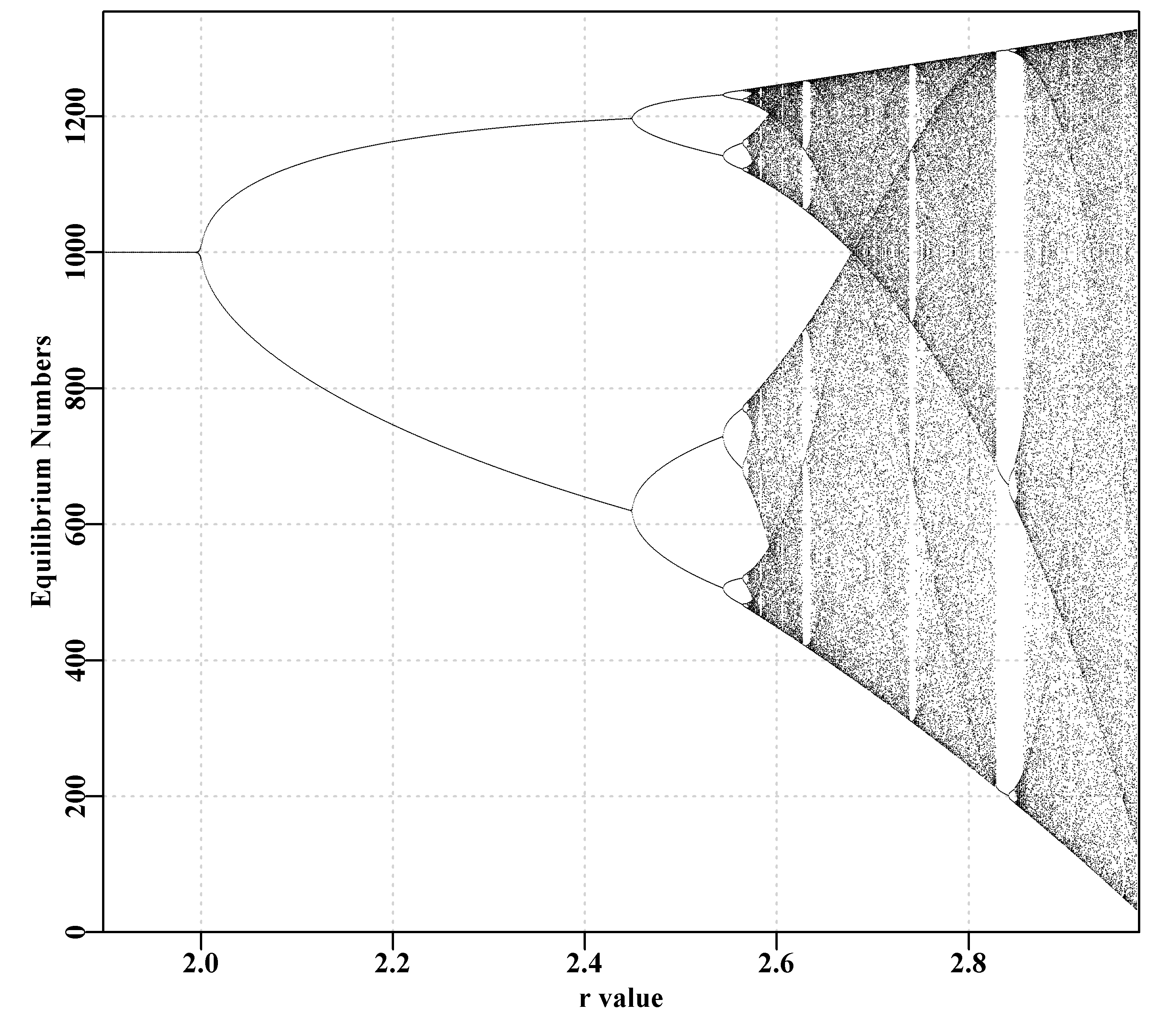
Figure 3.3: Schaefer model dynamics. A classical bifurcation diagram (May, 1976) plotting equilibrium dynamics against values of r, illustrating the transition from 2-, 4-, 8-cycle, and beyond, including chaotic behaviour.
3.1.5 The Effect of Fishing on Dynamics
If we set up a default discretelogistic() run to have an 8-cycle stable limit when catches are zero, we can apply different levels of constant catch to see how this may influence the dynamics. Here we have applied catches of 0, 50, 200, and 325 individuals (although the \(N_t\), \(K\), and \(C_t\) could also be in tonnes). Of course the initial value \(N_0\) must be greater than the catch but otherwise one is free to vary the values. In the four cases below we have assumed a \(p\) value of 1.0 (= Schaefer model), you could try \(p = 1e-08\) to explore the difference arising from using the equivalent to the Fox model.
 #Effect of catches on stability properties of discretelogistic
yrs=50; Kval=1000.0
nocatch <- discretelogistic(r=2.56,K=Kval,N0=500,Ct=0,Yrs=yrs)
catch50 <- discretelogistic(r=2.56,K=Kval,N0=500,Ct=50,Yrs=yrs)
catch200 <- discretelogistic(r=2.56,K=Kval,N0=500,Ct=200,Yrs=yrs)
catch300 <- discretelogistic(r=2.56,K=Kval,N0=500,Ct=300,Yrs=yrs)
We have put together a small function, plottime(), to simplify the repeated plotting of the final objects. We have also used the utility function parsyn() to aid with the syntax of the par() function for defining the bounds of a base graphics plot. Notice that producing such functions can simplify the subsequent code and I would recommend that individuals build up a collection of such useful functions that can be used with the function source() to introduce them to their own sessions (like a pre-package; do not forget to document your functions as you write them, RStudio even has an insert Roxygen skeleton command). Here, as catches increase one can see the dynamics begin to stabilize from 4- to 2-cycle, then asymptotic equilibrium. Notice that the mean stock size through time (the number at the bottom of each graph) declines as the constant catch increases.
 #Effect of different catches on n-cyclic behaviour Fig3.4
plottime <- function(x,ylab) {
   yrs <- nrow(x)
   plot1(x[,"year"],x[,"nt"],ylab=ylab,defpar=FALSE)
   avB <- round(mean(x[(yrs-40):yrs,"nt"],na.rm=TRUE),3)
   mtext(avB,side=1,outer=F,line=-1.1,font=7,cex=1.0)
} # end of plottime
 #the oma argument is used to adjust the space around the graph
par(mfrow=c(2,2),mai=c(0.25,0.4,0.05,0.05),oma=c(1.0,0,0.25,0))
par(cex=0.75, mgp=c(1.35,0.35,0), font.axis=7,font=7,font.lab=7)
plottime(nocatch,"Catch = 0")
plottime(catch50,"Catch = 50")
plottime(catch200,"Catch = 200")
plottime(catch300,"Catch = 300")
mtext("years",side=1,outer=TRUE,line=-0.2,font=7,cex=1.0) 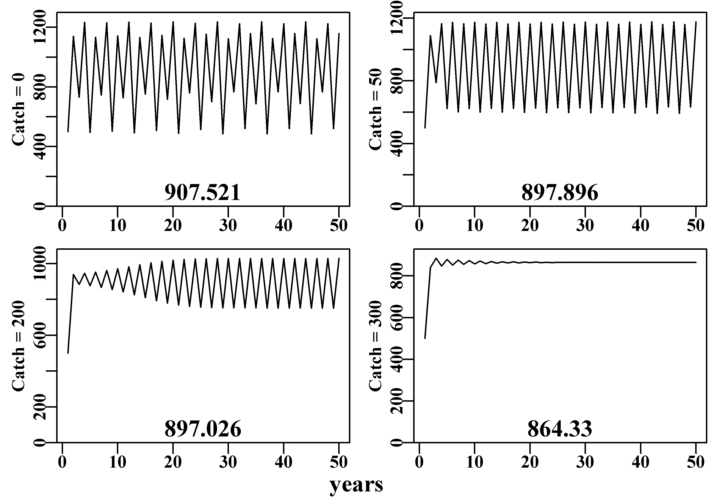
Figure 3.4: Schaefer model dynamics. The top-left plot depicts the expected unfished dynamics (8-cycle) while the next three plots, with decreasing average catches, illustrate the impact of the increased catches with no other factor changing.
We can do something very similar for the four phase plots. Here we have borrowed parts of the code from the MQMF:::plot.dynpop() function to define a small custom function to facilitate plotting four phase plots together.
 #Phase plot for Schaefer model Fig 3.5
plotphase <- function(x,label,ymax=0) { #x from discretelogistic
  yrs <- nrow(x)
  colnames(x) <- tolower(colnames(x))
  if (ymax[1] == 0) ymax <- getmax(x[,c(2:3)])
  plot(x[,"nt"],x[,"nt1"],type="p",pch=16,cex=1.0,ylim=c(0,ymax),
       yaxs="i",xlim=c(0,ymax),xaxs="i",ylab="nt1",xlab="",
       panel.first=grid(),col="darkgrey")
  begin <- trunc(yrs * 0.6) #last 40% of yrs = 20, when yrs=50
  points(x[begin:yrs,"nt"],x[begin:yrs,"nt1"],pch=18,col=1,cex=1.2)
  mtext(label,side=1,outer=F,line=-1.1,font=7,cex=1.2)
} # end of plotphase
par(mfrow=c(2,2),mai=c(0.25,0.25,0.05,0.05),oma=c(1.0,1.0,0,0))
par(cex=0.75, mgp=c(1.35,0.35,0), font.axis=7,font=7,font.lab=7)
plotphase(nocatch,"Catch = 0",ymax=1300)
plotphase(catch50,"Catch = 50",ymax=1300)
plotphase(catch200,"Catch = 200",ymax=1300)
plotphase(catch300,"Catch = 300",ymax=1300)
mtext("nt",side=1,outer=T,line=0.0,font=7,cex=1.0)
mtext("nt+1",side=2,outer=T,line=0.0,font=7,cex=1.0) 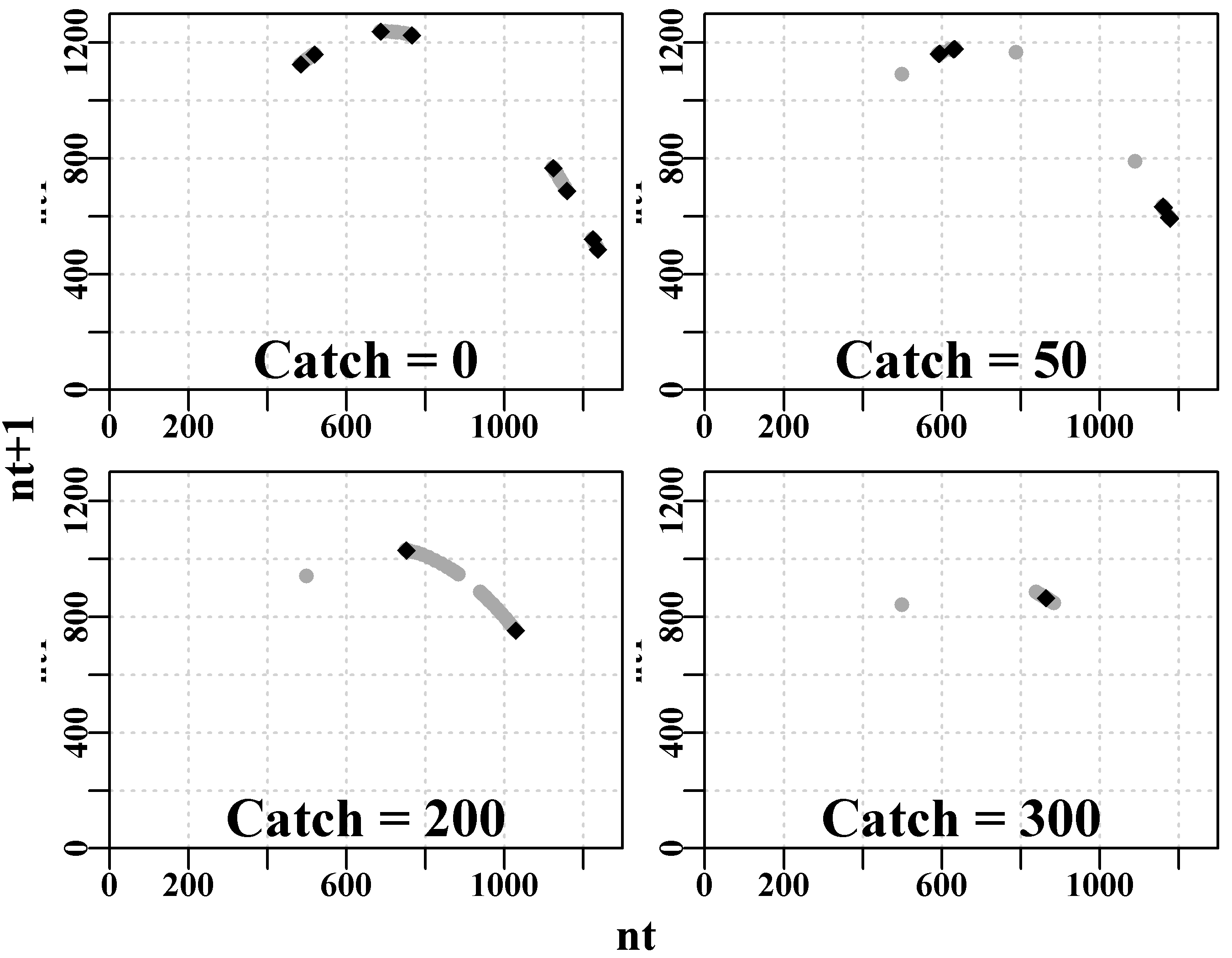
Figure 3.5: Schaefer model dynamics. Phase plots for each of the four constant catch scenarios.
Notice that as constant catches increase the maximum of the implied parabolic curve (strange attractor ) drops. Catches (\(\equiv\) predation) would appear to have a stabilizing influence on a stock’s dynamics. Whether this would be the case in nature would depend on whether the biology of the particular stock reflected the assumptions underlying the model used to describe the dynamics (for example, the Schaefer model assumes linear density-dependence operates in the population).
Hopefully now, it should be clear that even simple models can exhibit complex behaviour. We have only lightly touched on this subject but equally clearly, using R, it is possible to explore these ideas to whatever depth one wishes.
3.1.6 Determinism
All the models in this chapter exhibit deterministic dynamics, even the chaotic dynamics will follow the same trajectory if the starting conditions are repeated. In nature, of course, such deterministic behaviour would be rare. The models are always an abstraction of what may really be going on. The natural processes relating to productivity (natural mortality, growth, and reproduction) will all be variable through time in response to food availability, ecological interactions, and environmental influences such as temperature). Such variability within processes can be approximately included into models by including what is known as process error, which might be represented in equation form by:
\[\begin{equation} {N_{t+1}}={N_t}+{({r+\varepsilon_t}){N_t}}\left( 1-{{\left( \frac{N_t}{(K+\epsilon_t)} \right)}} \right) \tag{3.2} \end{equation}\]
where \(\varepsilon\) and \(\epsilon\) represent Normal random errors specific to each model parameter, which vary through time \(t\). Sometimes, in simulation, just one parameter will have variation added. As a population phenomenon, this would lead population numbers to follow trajectories that were not necessarily smooth, and, in a simulation, a single replicate would be insufficient to capture the potential range of the dynamics possible. The inclusion of such process errors in simulations would depend upon the purpose the modelling was being put to. Here, the intent is to explore the expectations of deterministic population dynamics, but one should always keep in mind that such models are only approximations and are intended to represent average behaviour.
3.2 Age-Structured Modelling Concepts
Of course the greatest simplification within the surplus production models we have just examined is that they ignore all aspects of age- and size-related differences in biology and behaviour. Such simplified models remain useful (see the chapter on Surplus Production Models), but in the face of acknowledged fishing gear selectivity (akin to predators having preferred prey) and differential growth and productivity at age, fisheries and other natural resource scientists often include age and or size in their models. Here we will only give such ideas an initial treatment as there are many other details about modelling dynamic processes required before embarking on such complexities in detail.
3.2.1 Survivorship in a Cohort
It is hopefully obvious that the survivorship of individuals, \(S\), between two time periods is simply the ratio of the numbers at \(t+1\) to the numbers at time \(t\) (keep in mind that numbers-at-age can be converted to mass-at-age or biomass-at-age when one know the weight-at-age relationship):
\[\begin{equation} S_t=\frac{{{N}_{t+1}}}{{{N}_{t}}}\text{ or }{{N}_{t+1}}={S_t}{N}_{t} \tag{3.3} \end{equation}\]
Such proportional reductions through time are suggestive of negative exponential growth. Given an instantaneous total mortality rate of \(Z\) (natural and fishing mortality combined), then the survivorship each year (that is the proportion surviving) is equal to \({e}^{-Z}\). This can be illustrated by setting up a simulated population with constant initial conditions and applying a vector of different instantaneous total mortality rates.
This would be equivalent to considering a single cohort recruiting as age 0+ individuals. Assuming no immigration, such a single-cohort population could only decline in numbers, which although seemingly trivially obvious is an important intuition when considering age-structured populations. The total mortality (usually denoted Z) is merely the sum of natural mortality (usually denoted M) and fishing mortality (usually denoted F). In the example below, notice that applying a Z = 0.05 leads to the population being greater than zero even after 50 years. Each of the cohort trajectories illustrated depicts an exponential or constant proportional decline in population size.
 #Exponential population declines under different Z. Fig 3.6
yrs <- 50;  yrs1 <- yrs + 1 # to leave room for B[0]
years <- seq(0,yrs,1)
B0 <- 1000        # now alternative total mortality rates
Z <- c(0.05,0.1,0.2,0.4,0.55)
nZ <- length(Z)
Bt <- matrix(0,nrow=yrs1,ncol=nZ,dimnames=list(years,Z))
Bt[1,] <- B0
for (j in 1:nZ) for (i in 2:yrs1) Bt[i,j] <- Bt[(i-1),j]*exp(-Z[j])
plot1(years,Bt[,1],xlab="Years",ylab="Population Size",lwd=2)
if (nZ > 1) for (j in 2:nZ) lines(years,Bt[,j],lwd=2,col=j,lty=j)
legend("topright",legend=paste0("Z = ",Z),col=1:nZ,lwd=3,
bty="n",cex=1,lty=1:5) 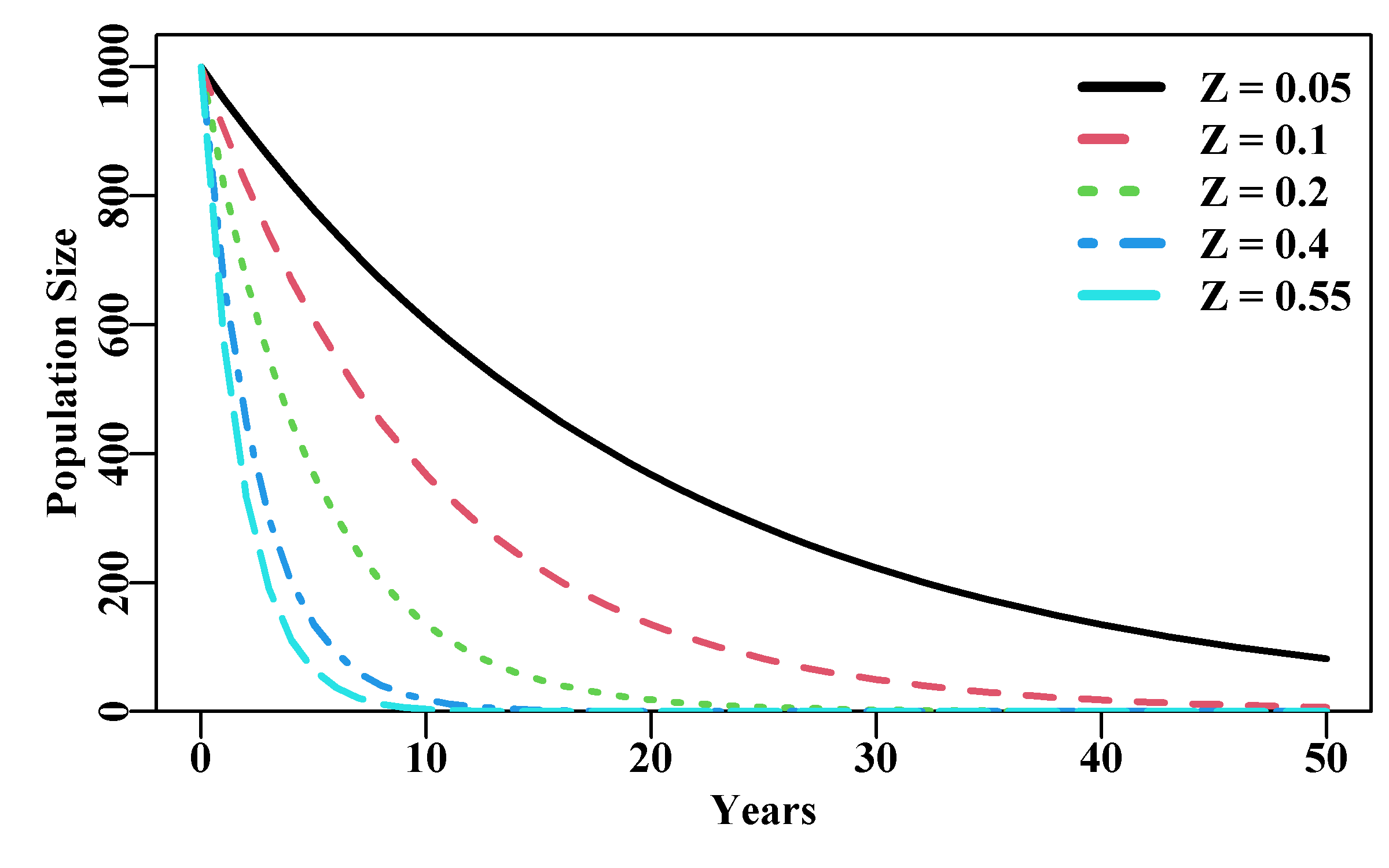
Figure 3.6: Exponential population declines under different levels of total mortality. The top curve is Z = 0.05 and the steepest curve is Z = 0.55.
3.2.2 Instantaneous vs Annual Mortality Rates
In the previous section we worked with what are known as instantaneous rates. They could be used to generate survivorship rates in terms of the proportion expected to survive after a year of a given instantaneous mortality rate. The idea behind an instantaneous mortality rate is that it is the mortality applied over infinitesimally small time periods.
We already know the annual proportion surviving:
\[\begin{equation} S={e}^{-Z} \tag{3.4} \end{equation}\]
Thus, the proportion that die (\(A\)) over the year is described by:
\[\begin{equation} A=1-{e}^{-Z} \tag{3.5} \end{equation}\]
If we only consider the instantaneous fishing mortality rate, F and ignore the natural mortality rate, then the proportion dying is known as the harvest rate, H.
\[\begin{equation} H=1-{e}^{-F} \tag{3.6} \end{equation}\]
If we know the annual harvest rate we can back transform that to estimate the instantaneous fishing mortality rate.
\[\begin{equation} F=-\log{(1-H)} \tag{3.7} \end{equation}\]
where \(\log\) denotes the natural log or logs to base e.
It can sometimes seem difficult to obtain an intuitive grasp of what instantaneous rates imply. This difficulty may be reduced if we illustrate how instantaneous rates can be derived. Starting with a population of 1000 individuals we can assume an annual removal rate of 0.5 meaning only 500 would survive the year. By substituting the total annual mortality rate into the last equation we can estimate the instantaneous total mortality rate to be \(-\log(1 - 0.5) = 0.693147\). If we approximate the time steps this level needs to be applied over to obtain the total of 50% surviving by using two 6 monthly periods, we would need to divide the 0.693147 by 2.0 and apply that mortality rate twice. Similarly, if the time steps were monthly, we would divide by 12 and apply the result 12 times. While each month could hardly be termed instantaneous this would be the period over which the approximate instantaneous rate (0.693147/12) of mortality would be applied. Such a re-scaling could occur with smaller and smaller time intervals until the intervals were small enough that the result was not significantly different from the expected 500 individual remaining at the end of a year, Table(3.3).
As becomes apparent, the shorter the time interval over which the approximate instantaneous rate is applied the closer the final value comes to the expected 0.5 of 1000 (i.e. 500). Hopefully, playing around with this code will assist you in gaining intuitions about the notion of instantaneous rates of mortality.
Annual rates can be plotted against instantaneous rates of mortality to illustrate the difference between the two. Note that up to about an instantaneous rate of 0.18 the annual harvest rate has approximately the same value. It should be clear that it is not possible to get a harvest rate greater than 1.0 (equivalent to capturing >100% of the exploitable biomass). High harvest rates begin to appear to be implausible and if they occur when fitting a fisheries model they should really need to be defended before being accepted. Instantaneous rates, on the other hand, can obviously be over 1.0, but ideally such an event should no longer be misunderstood.
 #Prepare matrix of harvest rate vs time to appoximate F
Z <- -log(0.5)
timediv <- c(2,4,12,52,365,730,2920,8760,525600)
yrfrac <- 1/timediv
names(yrfrac) <- c("6mth","3mth","1mth","1wk","1d","12h",
                   "3h","1h","1m")
nfrac <- length(yrfrac)
columns <- c("yrfrac","divisor","yrfracH","Remain")
result <- matrix(0,nrow=nfrac,ncol=length(columns),
                 dimnames=list(names(yrfrac),columns))
for (i in 1:nfrac) {
   timestepmort <- Z/timediv[i]
   N <- 1000
   for (j in 1:timediv[i]) N <- N * (1-timestepmort)
   result[i,] <- c(yrfrac[i],timediv[i],timestepmort,N)
} | yrfrac | divisor | yrfracH | Remain | |
|---|---|---|---|---|
| 6mth | 0.5000000000 | 2 | 0.34657359 | 426.9661 |
| 3mth | 0.2500000000 | 4 | 0.17328680 | 467.1104 |
| 1mth | 0.0833333333 | 12 | 0.05776227 | 489.6953 |
| 1wk | 0.0192307692 | 52 | 0.01332975 | 497.6748 |
| 1d | 0.0027397260 | 365 | 0.00189903 | 499.6706 |
| 12h | 0.0013698630 | 730 | 0.00094952 | 499.8354 |
| 3h | 0.0003424658 | 2920 | 0.00023738 | 499.9589 |
| 1h | 0.0001141553 | 8760 | 0.00007913 | 499.9863 |
| 1m | 0.0000019026 | 525600 | 0.00000132 | 499.9998 |
 #Annual harvest rate against instantaneous F, Fig 3.7
Fi <- seq(0.001,2,0.001)
H <- 1 - exp(-Fi)
parset()  # a wrapper for simplifying defining the par values
plot(Fi,H,type="l",lwd=2,panel.first=grid(),
     xlab="Instantaneous Fishing Mortality F",
     ylab="Annual Proportion Mortality H")
lines(c(0,1),c(0,1),lwd=2,lty=2,col=2) 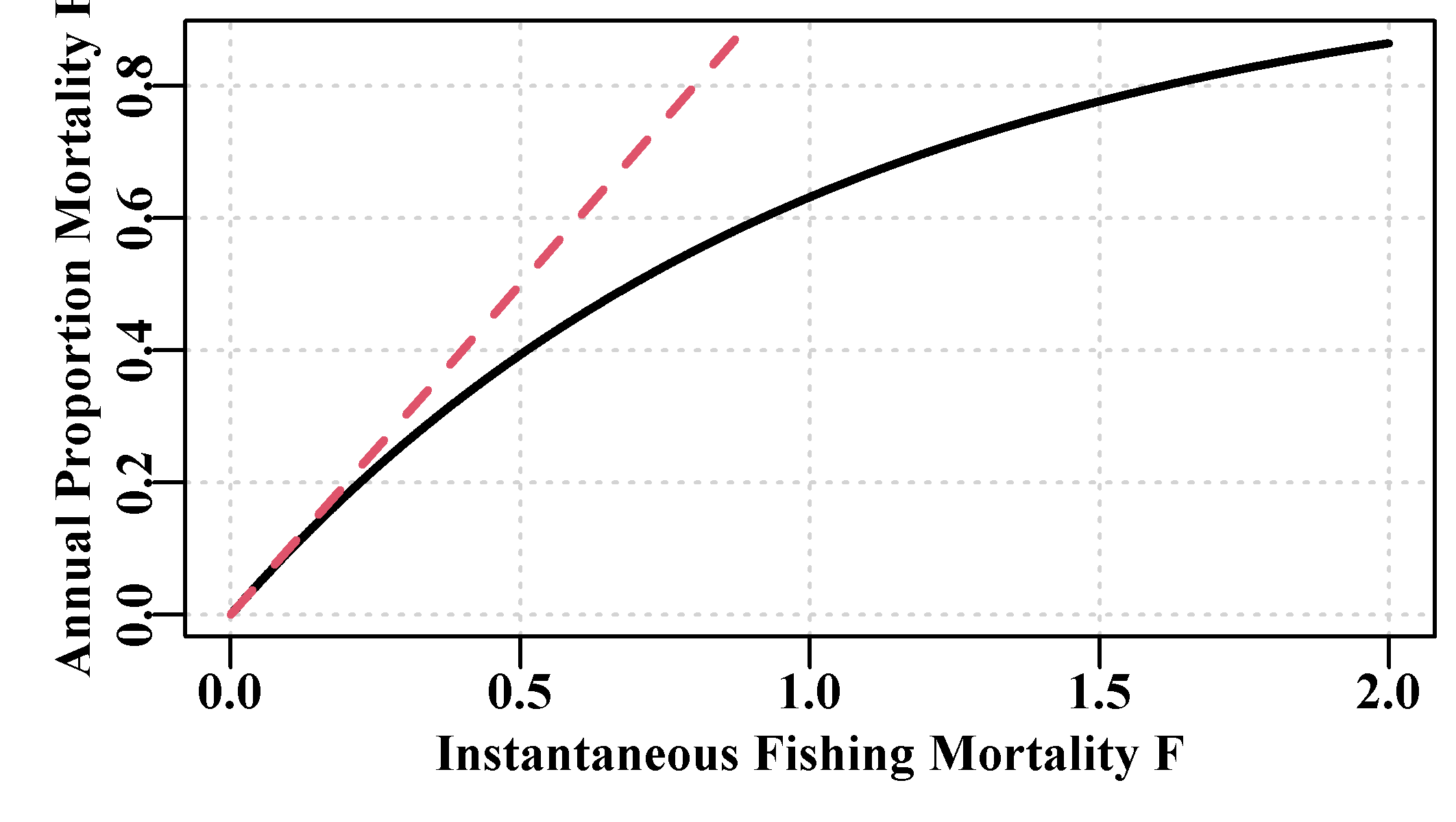
Figure 3.7: The relationship between the instantaneous fishing mortality rate (solid line) and the annual fishing mortality or annual harvest rate (dashed line). The values diverge at values of F greater than about 0.2.
3.3 Simple Yield per Recruit
We know that once a cohort recruits to a stock its numbers can only decrease (assuming no immigration). Take care over the concept of “recruitment”, it can mean the post-larval arrival into the stock, however, it can also refer to when individuals become available or vulnerable to a fishery. Here we are concerned with post-larval arrival. We will deal with recruitment to a fishery when we consider the notion of selectivity and availability below and in Static Models. Interestingly, while numbers are expected to decrease through time, given that individuals can grow in size and weight, we do not yet know if the mass of the members of a cohort always decreases through time or if it increases first and then decreases as eventually all the individuals die.
The question of whether the mass of a cohort can increase for some years, even as its numbers decline was first explored because of a simplistic but common intuition about the relationship between catch and effort. It may seem obvious that the catch of a fish species landed will always increase with an increase in fishing effort, but that is short-term thinking. This seemingly obvious notion was refuted before 1930, and was illustrated nicely by some published work by Russell (1942), who demonstrated that the maximum on-going catch from a fishery need not necessarily arise from the maximum effort (or the maximum fishing mortality ). This was not just an academic question but directly related to the management of fisheries. Once it was realized that it was possible to over-fish and even collapse a fish stock, which was only formally recognized at the start of the 20th century (Garstang, 1900), then how best to manage fisheries became an important question. Attempts were made to manage fisheries by attempting to manage the total effort applied. An argument in support of this derived from the notions of yield-per-recruit (YPR), which mathematically followed the fate, in terms of numbers and mass, of cohorts under different levels of imposed fishing mortality; fishing mortality was taken to be directly related to the effort applied. The notion of ‘per-recruit’ implied it followed individual cohorts and to begin with had the objective of maximizing the yield possible from each recruit.
We will repeat Russell’s (1942) example to illustrate the ideas behind YPR. Russell’s example only concerned itself with fishing mortality, which is the same as assuming no natural mortality (M was ignored). For this simple YPR we will also ignore natural mortality and just apply a series of constant harvest rates each year to calculate the numbers-at-age (equivalent to Equ(3.3)), then we will use a weight-at-age multiplied by the numbers-at-age series to calculate the weight of the catch-at-age, from which we can obtain the total expected catch.
 # Simple Yield-per-Recruit see Russell (1942)
age <- 1:11;  nage <- length(age); N0 <- 1000  # some definitions
 # weight-at-age values
WaA <- c(NA,0.082,0.175,0.283,0.4,0.523,0.7,0.85,0.925,0.99,1.0)
 # now the harvest rates
H <- c(0.01,0.06,0.11,0.16,0.21,0.26,0.31,0.36,0.55,0.8)
nH <- length(H)
NaA <- matrix(0,nrow=nage,ncol=nH,dimnames=list(age,H)) # storage
CatchN <- NaA;  CatchW <- NaA      # define some storage matrices
for (i in 1:nH) {                # loop through the harvest rates
   NaA[1,i] <- N0  # start each harvest rate with initial numbers
   for (age in 2:nage) {  # loop through over-simplified dynamics
      NaA[age,i] <- NaA[(age-1),i] * (1 - H[i])
      CatchN[age,i] <- NaA[(age-1),i] - NaA[age,i]
   }
   CatchW[,i] <- CatchN[,i] * WaA
}                      # transpose the vector of total catches to
totC <- t(colSums(CatchW,na.rm=TRUE))   # simplify later printing
The impact of the different harvest rates on the age-structure of the population is apparent in both the numbers-at-age and the weight-at-age in the catch. As the harvest rate increases the numbers-at-age in the older classes becomes more and more reduced, and similarly for the catch-at-age. For the higher harvest rates the stock becomes dependent upon the recent recruitment rather than any accumulation of numbers and biomass in the older classes.
| 0.01 | 0.06 | 0.11 | 0.16 | 0.21 | 0.26 | 0.31 | 0.36 | 0.55 | 0.8 | |
|---|---|---|---|---|---|---|---|---|---|---|
| 1 | 1000 | 1000 | 1000 | 1000 | 1000 | 1000 | 1000 | 1000 | 1000.0 | 1000.0 |
| 2 | 990 | 940 | 890 | 840 | 790 | 740 | 690 | 640 | 450.0 | 200.0 |
| 3 | 980 | 884 | 792 | 706 | 624 | 548 | 476 | 410 | 202.5 | 40.0 |
| 4 | 970 | 831 | 705 | 593 | 493 | 405 | 329 | 262 | 91.1 | 8.0 |
| 5 | 961 | 781 | 627 | 498 | 390 | 300 | 227 | 168 | 41.0 | 1.6 |
| 6 | 951 | 734 | 558 | 418 | 308 | 222 | 156 | 107 | 18.5 | 0.3 |
| 7 | 941 | 690 | 497 | 351 | 243 | 164 | 108 | 69 | 8.3 | 0.1 |
| 8 | 932 | 648 | 442 | 295 | 192 | 122 | 74 | 44 | 3.7 | 0.0 |
| 9 | 923 | 610 | 394 | 248 | 152 | 90 | 51 | 28 | 1.7 | 0.0 |
| 10 | 914 | 573 | 350 | 208 | 120 | 67 | 35 | 18 | 0.8 | 0.0 |
| 11 | 904 | 539 | 312 | 175 | 95 | 49 | 24 | 12 | 0.3 | 0.0 |
| 0.01 | 0.06 | 0.11 | 0.16 | 0.21 | 0.26 | 0.31 | 0.36 | 0.55 | 0.8 | |
|---|---|---|---|---|---|---|---|---|---|---|
| 2 | 0.82 | 4.92 | 9.02 | 13.12 | 17.22 | 21.32 | 25.42 | 29.52 | 45.10 | 65.60 |
| 3 | 1.73 | 9.87 | 17.13 | 23.52 | 29.03 | 33.67 | 37.43 | 40.32 | 43.31 | 28.00 |
| 4 | 2.77 | 15.00 | 24.66 | 31.95 | 37.09 | 40.29 | 41.77 | 41.73 | 31.52 | 9.06 |
| 5 | 3.88 | 19.93 | 31.02 | 37.93 | 41.42 | 42.14 | 40.74 | 37.75 | 20.05 | 2.56 |
| 6 | 5.02 | 24.50 | 36.10 | 41.66 | 42.78 | 40.78 | 36.75 | 31.59 | 11.80 | 0.67 |
| 7 | 6.66 | 30.82 | 43.00 | 46.84 | 45.23 | 40.39 | 33.94 | 27.06 | 7.10 | 0.18 |
| 8 | 8.00 | 35.18 | 46.47 | 47.78 | 43.39 | 36.29 | 28.44 | 21.03 | 3.88 | 0.04 |
| 9 | 8.62 | 35.99 | 45.01 | 43.67 | 37.30 | 29.22 | 21.35 | 14.65 | 1.90 | 0.01 |
| 10 | 9.14 | 36.21 | 42.87 | 39.26 | 31.54 | 23.15 | 15.77 | 10.03 | 0.92 | 0.00 |
| 11 | 9.14 | 34.38 | 38.54 | 33.31 | 25.17 | 17.30 | 10.99 | 6.49 | 0.42 | 0.00 |
| 0.01 | 0.06 | 0.11 | 0.16 | 0.21 | 0.26 | 0.31 | 0.36 | 0.55 | 0.8 |
|---|---|---|---|---|---|---|---|---|---|
| 55.8 | 246.8 | 333.8 | 359.1 | 350.2 | 324.5 | 292.6 | 260.2 | 166 | 106.1 |
If we use the MQMF plot1() function to plot out the total weight of catch against the harvest rate, we can immediately see that there is indeed an optimum harvest rate in terms of yield produced and that it is not the maximum used. Catches do not always increase if effort is allowed to increase. If the harvest rate is very low, then too few animals are caught to make up a significant catch. However, the yield rapidly increases with harvest rate and tails down more slowly as the harvest rate that generates the maximum yield is exceeded.
 #Use MQMF::plot1 for a quick plot of the total catches. Figure 3.8
plot1(H,totC,xlab="Harvest Rate",ylab="Total Yield",lwd=2) 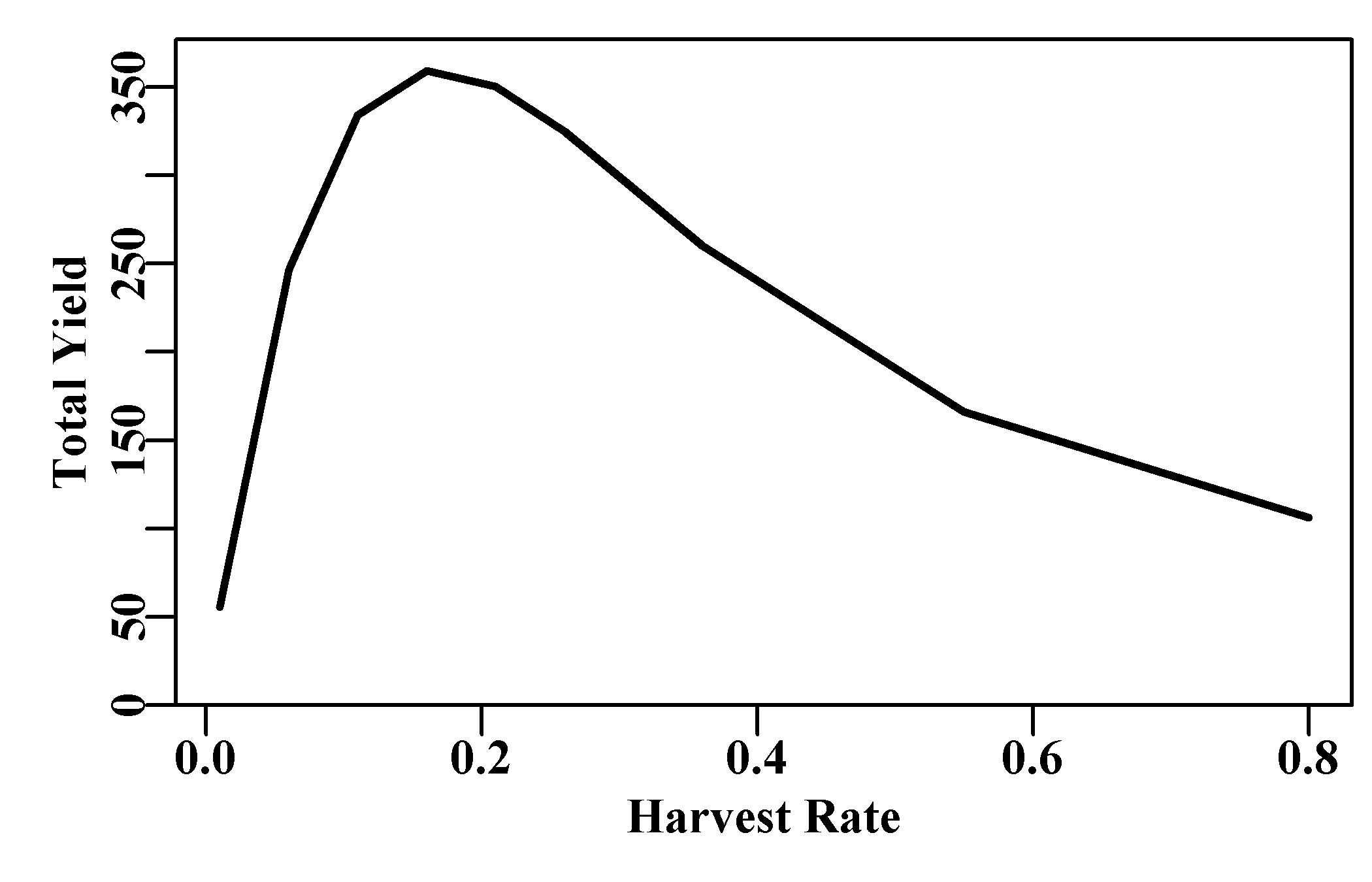
Figure 3.8: A simplified yield-per-recruit analysis that ignores natural mortality, selectivity-at-age, or any other influences. This analysis uses some weight-at-age data from Russell, 1942 although a wider array of harvest rates were examined than just the two by Russell.
As a quick illustration of the impact of different harvest rates this example was successful in 1942. A fuller treatment of yield-per-recruit needs to account for natural mortality in the dynamics and differential mortality rates by age brought about by gear selectivity.
3.3.1 Selectivity in Yield-per-Recruit
Usually, in a fully age-structured fisheries model one would implement a selectivity function to describe the different vulnerability of each age-class (or size-class) to a particular fishing gear. As the fish get older (or bigger), they recruit more and more to the fishery until they are completely vulnerable to fishing should it occur where they are. Normally, the parameters of such selectivity curves are obtained in the process of fitting the age-structured model to data from the fishery. Here, however, we will merely be attributing values (see more details of selectivity in the Static Models chapter). Early YPR analyses often used what is known as knife-edged selectivity, implying that fish became 100% vulnerable to gear at a particular age. Here however, we will implement a more realistic, yet simple, selectivity curve of vulnerability against age. There are many different equations used to describe the selectivity characteristics of different fishing gears but an extremely common one used for trawl gear is the standard logistic or S-shaped curve, which can also have a number of formulaic expressions. An equation commonly used to describe the logistic shape of selectivity with age, \(s_a\), or size, and also maturity at age or size is defined as:
\[\begin{equation} {{s}_{a}}=\frac{1}{1+{{({{e}^{(\alpha +\beta a)}})}^{-1}}}=\frac{{{e}^{(\alpha +\beta a)}}}{1+{{e}^{(\alpha +\beta a)}}} \tag{3.8} \end{equation}\]
where \(\alpha\) and \(\beta\) are the logistic parameters, and \(-\alpha/\beta\) is the age at a selectivity of 0.5 (50%). The inter-quartile distance (literally quantile 25% to quantile 75%; a measure of the gradient of the logistic curve) is defined as \(IQ = 2 \log{(3)} /\beta\) (see the MQMF function mature() for an implementation of this function). Generally, in age-structured modelling one needs length- or age-composition data so that the gear selectivity combined with fishery availability can be estimated directly. When working with yield-per-recruit calculations the usual reason to include a form of selectivity is to determine the optimum age at which to begin applying fishing mortality. In management terms this could be used to determine trawl or gillnet mesh sizes. This is the reason that knife-edged selectivity was often used, which would identify the age below which there is no selection and above which there is 100% selection. This is implemented in the MQMF function logist() (which uses a different formulation) but not in mature(). Knife-edged selectivity does not tend to be used in full age-structured stock assessment models.
 #Logistic S shaped cureve for maturity
ages <- seq(0,50,1)
sel1 <- mature(-3.650425,0.146017,sizeage=ages) #-3.65/0.146=25
sel2 <- mature(-6,0.2,ages)
sel3 <- mature(-6,0.24,ages)
plot1(ages,sel1,xlab="Age Yrs",ylab="Selectivity",cex=0.75,lwd=2)
lines(ages,sel2,col=2,lwd=2,lty=2)
lines(ages,sel3,col=3,lwd=2,lty=3)
abline(v=25,col="grey",lty=2)
abline(h=c(0.25,0.5,0.75),col="grey",lty=2)
legend("topleft",c("25_15.04","30_10.986","25_9.155"),col=c(1,2,3),
lwd=3,cex=1.1,bty="n",lty=1:3) 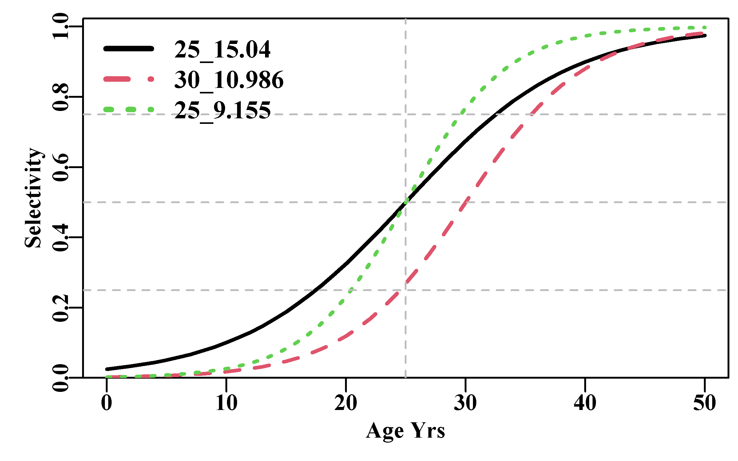
Figure 3.9: Examples of the logistic S-shaped curve using the mature() function. The legend consists of the L50 and the IQ for each curve with their parameters defined in the code.
3.3.2 The Baranov Catch Equation
Equ(3.4) described survivorship following the combination of fishing and natural mortality, but the simple \(Z\) for total mortality implied that all fish suffered the same fishing mortality. If we are to take account of selectivity then we need to consider fishing mortality at age.
\[\begin{equation} S_{a,t}=e^{-(M + {s_a}{F_t})} \tag{3.9} \end{equation}\]
where \(S_{a,t}\) is the survivorship of fish aged \(a\) in year \(t\), \(M\) is the natural mortality (assumed constant through time), \(s_a\) is the selectivity for age \(a\), and \(F_t\) is known as the fully selected fishing mortality in year \(t\).
Once we know the numbers surviving \({S_t}{N_t}\), then the numbers dying are obviously the difference between time periods. The total number dying within a cohort from one time period to the next can be described by:
\[\begin{equation} N_{z}=N_{t}-N_{t+1} \tag{3.10} \end{equation}\]
If we replace the Nt+1 with the survivorship equation, we get the complement of the survivorship equation, which describes the total numbers dying between time periods:
\[\begin{equation} N_{a,z}=N_{a,t}-N_{a,t}{e}^{-(M+{s_a}{F_t})}=N_{a,t}(1-{e}^{-(M+{s_a}{F_t})}) \tag{3.11} \end{equation}\]
Here \(N_{a,z}\) is the numbers of age \(a\) dying. Of course, not all of those dying fish were taken as catch, some would have died naturally, but also some that would have died naturally would have been caught. The separation of mortality into \(M\), the assumed constant across ages natural mortality, and \(F_t\) the fully selected mortality due to the fishing effort, which can vary depending in which time period \(t\) it is imposed allows the catch and survivorship to be calculated. For simplicity \({s_a}{F_t}\) can be designated as \(F_{a,t}\). The assumption that it is possible to make this separation is a vital component of age- and size-structured stock assessment models. Using instantaneous rates, the numbers that die due to fishing mortality rather than natural mortality are described by the fraction \(F_{a,t}/(M+F_{a,t})\), and if that is included in equation Equ(3.11), we find that we have derived what is known as the Baranov catch equation (Quinn, 2003; Quinn and Deriso, 1999), which is now generally used in fisheries modelling to estimate the numbers taken in the catch. It is used to follow the fate of individual cohorts, which if summed across ages gives the total catches:
\[\begin{equation} {{\hat{C}}_{a,t}}=\frac{{F}_{a,t}}{M+{F}_{a,t}}{{N}_{a,t}}\left( 1-{{e}^{-\left( M+{{F}_{a,t}} \right)}} \right) \tag{3.12} \end{equation}\]
where \(\hat{C}_{a,t}\) is the expected catch at age \(a\) in year \(t\), \(F_{a,t}\) is the instantaneous fishing mortality rate at age \(a\) in year \(t\) (\({s_a}{F_t}\)), \(M\) is the natural mortality rate (assumed constant across age-classes), and \(N_{a,t}\) is the numbers at age \(a\) in year \(t\). This equation is implemented in the MQMF function bce().
 # Baranov catch equation
age <- 0:12;  nage <- length(age)
sa <-mature(-4,2,age) #selectivity-at-age
H <- 0.2;  M <- 0.35
FF <- -log(1 - H)#Fully selected instantaneous fishing mortality
Ft <- sa * FF     # instantaneous Fishing mortality-at-age
N0 <- 1000
out <- cbind(bce(M,Ft,N0,age),"Select"=sa) # out becomes Table 3.7 | Nt | N-Dying | Catch | Select | |
|---|---|---|---|---|
| 0 | 1000.000 | 0.018 | ||
| 1 | 686.191 | 291.645 | 22.164 | 0.119 |
| 2 | 432.501 | 192.368 | 61.322 | 0.500 |
| 3 | 250.395 | 116.618 | 65.488 | 0.881 |
| 4 | 141.728 | 66.827 | 41.840 | 0.982 |
| 5 | 79.943 | 37.766 | 24.018 | 0.998 |
| 6 | 45.071 | 21.298 | 13.574 | 1.000 |
| 7 | 25.409 | 12.007 | 7.655 | 1.000 |
| 8 | 14.325 | 6.769 | 4.316 | 1.000 |
| 9 | 8.075 | 3.816 | 2.433 | 1.000 |
| 10 | 4.553 | 2.151 | 1.372 | 1.000 |
| 11 | 2.567 | 1.213 | 0.773 | 1.000 |
| 12 | 1.447 | 0.684 | 0.436 | 1.000 |
3.3.3 Growth and Weight-at-Age
To obtain the catch as mass (i.e. the weight of catch) the numbers-at-age in the catch need to be multiplied by the weight-at-age. The weight-at-age can either be a vector of mean weight observations from a particular fishery for each particular year (Beverton and Holt, 1957) or, more commonly, a standard weight-at-age equation that derives from the von Bertalanffy growth curve, which starts as length-at-age.
\[\begin{equation} L_{a}=L_{\infty}(1-e^{(-K(a-t_0))}) \tag{3.13} \end{equation}\]
where \(L_a\) is the length-at-age \(a\), \(L_{\infty}\) is the mean maximum length-at-age, \(K\) is the coefficient, which determines how quickly \(L_{\infty}\) is achieved, and \(t_0\) is the hypothetical age at length zero. This is implemented in the MQMF function vB(). The assumption is made that there is a power relationship between length-at-age and weight-at-age so two more parameters are added to give:
\[\begin{equation} \begin{split} {W_a} &= {\alpha}{L_a}^{b}=w_a(1-e^{(-K(a-t_0))})^{b} \\ {\log{(W_a)}} &= \log{(\alpha)}+{b}{L_a} \end{split} \tag{3.14} \end{equation}\]
where \(\alpha\) is a constant, wa is (\({\alpha}{L_{\infty}}\)), and b is the exponent, which usually approximates to a value of 3.0 (size measures are two-dimensional while weight measures are three dimensional). The log-transformed version is, of course, linear. In the Static Models chapter we will see how parameters for such models can be estimated.
3.4 Full Yield-per-Recruit
Pulling all of this together means we can produce a much more complete yield-per-recruit (YPR) analysis. A standard YPR analysis assumes constant recruitment which means we can follow the fate of a single cohort and still capture the required details. Of course, recruitment is not a constant so this approach is considered to be based upon long-run or equilibrium conditions. Ignoring variation and stochasticity in this way means that any conclusions drawn, with regard to potential productivity and resulting management decisions, need to be treated with caution (in fact, with great caution). But these approaches were developed when fisheries analyses were all deterministic and assumed to be at equilibrium, the implications of uncertainty had not yet been explored (Beverton and Holt, 1957).
It makes sense to do such analyses when the objective is to maximize yield. But the assumption of constant recruitment and the lack of attention paid to uncertainty means these analyses are generally not conservative. Attempts were made to improve on the recommendations that flowed from YPR analyses with one of the more useful being the advent of F0.1 (pronounced F zero point one). This is defined as the harvest rate at which the rate of increase in yield is 1/10 that at the origin of a yield curve (Hilborn and Walters, 1992). The advantage of \(F_{0.1}\) is that a relatively large reduction in fishing effort and can lead to only a small loss in yield. This can improve both the economics and the sustainability of a fishery. Nevertheless, essentially the use of \(F_{0.1}\) remains an empirical rule which was found to be more sustainable in practice than either Fmax (the point of maximum yield) and usually better than Fmsy (the fishing mortality that, at equilibrium, would generate the MSY).
 # A more complete YPR analysis
age <- 0:20;  nage <- length(age) #storage vectors and matrices
laa <- vB(c(50.0,0.25,-1.5),age) # length-at-age
WaA <- (0.015 * laa ^ 3.0)/1000  # weight-at-age as kg
H <- seq(0.01,0.65,0.05);  nH <- length(H)
FF <- round(-log(1 - H),5)  # Fully selected fishing mortality
N0 <- 1000
M <- 0.1
numt <- matrix(0,nrow=nage,ncol=nH,dimnames=list(age,FF))
catchN <- matrix(0,nrow=nage,ncol=nH,dimnames=list(age,FF))
as50 <- c(1,2,3)
yield <- matrix(0,nrow=nH,ncol=length(as50),dimnames=list(H,as50))
for (sel in 1:length(as50)) {
   sa <- logist(as50[sel],1.0,age)  # selectivity-at-age
   for (harv in 1:nH) {
      Ft <- sa * FF[harv]      # Fishing mortality-at-age
      out <- bce(M,Ft,N0,age)
      numt[,harv] <- out[,"Nt"]
      catchN[,harv] <- out[,"Catch"]
      yield[harv,sel] <- sum(out[,"Catch"] * WaA,na.rm=TRUE)
   } # end of harv loop
} # end of sel loop
#A full YPR analysis Figure 3.10
plot1(H,yield[,3],xlab="Harvest Rate",ylab="Yield",cex=0.75,lwd=2)
lines(H,yield[,2],lwd=2,col=2,lty=2)
lines(H,yield[,1],lwd=2,col=3,lty=3)
legend("bottomright",legend=as50,col=c(3,2,1),lwd=3,bty="n",
cex=1.0,lty=c(3,2,1)) 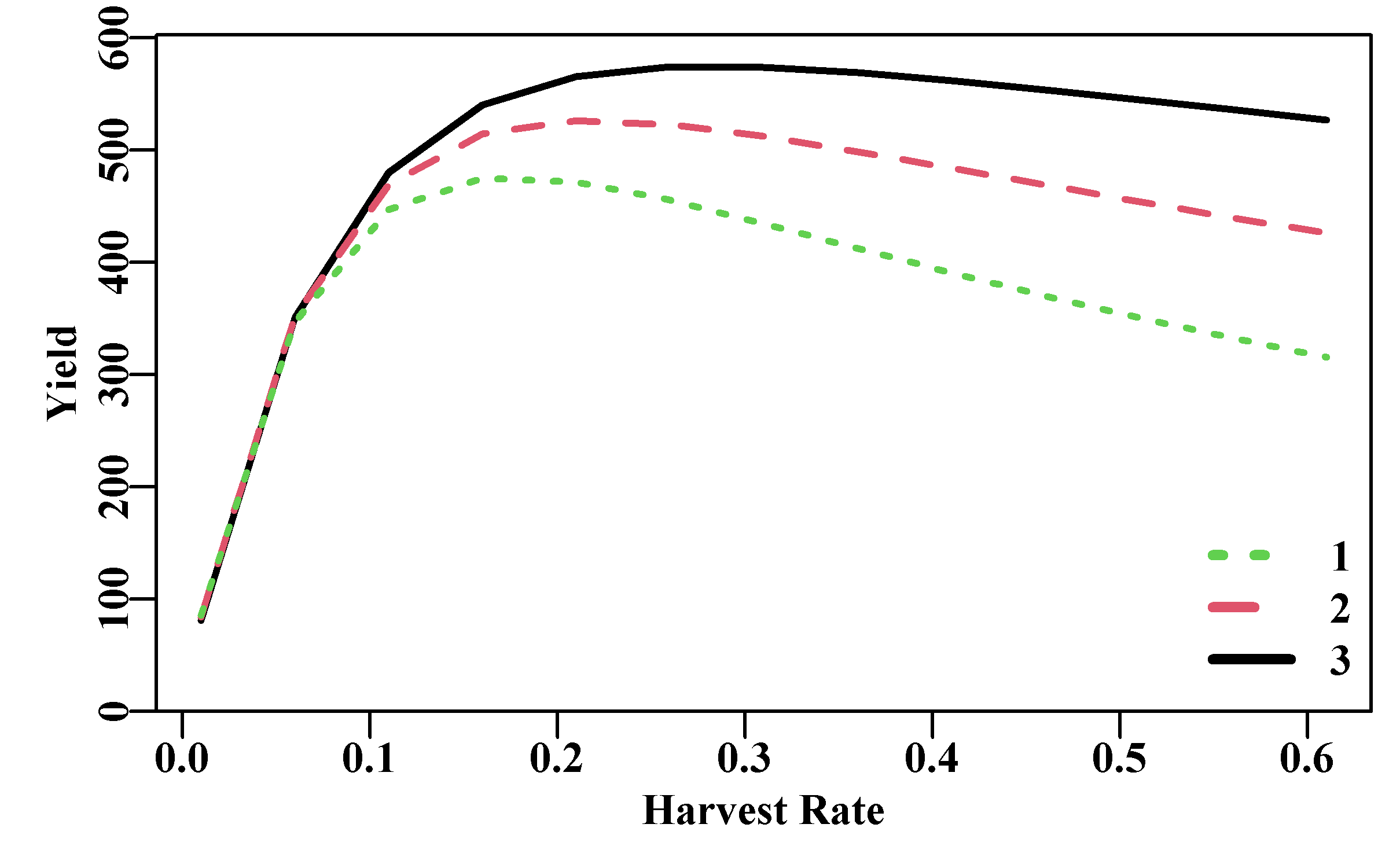
Figure 3.10: The effect on the total equilibrium yield of applying different harvest rates and different ages of first exploitation. The legend identifies the different age of first exploitation.
These detailed analyses, allowing for selectivity, weight-at-age, and natural mortality, provide a more accurate, albeit still deterministic, representation of the potential yield from a fishery under different conditions. Once uncertainty and natural variation are taken into account, even just approximately by using \(F_{0.1}\), then a YPR analysis can still provide some useful insights into the productive capacity of particular fisheries. of course, these days, onbe would be more likely to conduct a profit-per-recruit analysis, but the principles remain the same.
| 1 | 2 | 3 | |
|---|---|---|---|
| 0.01 | 85.82 | 84.152 | 81.136 |
| 0.06 | 347.12 | 352.465 | 350.567 |
| 0.11 | 447.07 | 469.250 | 480.134 |
| 0.16 | 475.15 | 514.595 | 540.249 |
| 0.21 | 471.99 | 526.522 | 565.880 |
| 0.26 | 455.84 | 522.962 | 574.288 |
| 0.31 | 434.88 | 512.360 | 573.986 |
| 0.36 | 412.72 | 498.720 | 569.223 |
| 0.41 | 390.96 | 483.969 | 562.163 |
| 0.46 | 370.25 | 469.031 | 553.935 |
| 0.51 | 350.83 | 454.348 | 545.146 |
| 0.56 | 332.72 | 440.100 | 536.113 |
| 0.61 | 315.81 | 426.329 | 526.995 |
3.5 Concluding Remarks
We have used relatively simple population models to illustrate numerous ideas from fisheries and ecology. Importantly, the focus was on simulation models rather than fitting models to data (see the next chapter on Model Parameter Estimation). Simulation models would usually include uncertainty in the model parameter values, however, as with many of the subjects given only an introductory treatment here, a more thorough treatment would entail a book in itself. Nevertheless, by exploring the implications of imposing a range of parameter values on the various models considered, the properties and implied dynamics of these models can be laid bare. As such, simulation studies are a vital tool in the modelling of any natural processes. Equally important, however, is using such simulations with plausible or realistic combinations of parameters. It is useful to understand the mathematical properties of all models but, naturally, the prime interest is when the models take on realistic values and might be found in nature.
The intuitions obtained when using any population model or their components have value in understanding any future work, but, of course, the context and assumptions in each of the models illustrated (especially the relatively simple models) have always to be kept in mind. The surprising thing is that even simple models can sometimes provide insight into various natural processes.
In this chapter we have only considered simple population models but we could equally well use R to explore interactions between species in processes such as competition, predation, parasitism, symbiosis, and others. All the early models (Lotka, 1925; Volterra, 1927; Gause, 1934) considered populations with no spatial structure. Using R it would be relatively straight forward to increase the complexity of such models and include spatial details such as explored experimentally by Huffaker (1958). Some of Huffaker’s later experimental predator-prey arrangements lasted for 490 days. In such cases, simulation studies could become very useful for expanding on what explorations are possible. Such interesting work would need to be a part of a different book as here we still have many other areas to explore and discuss in the field of fisheries.
The use of R as the tool for conducting such simulations makes the analyses somewhat more abstract than laying the parameter manipulations out on a spreadsheet. Nevertheless, the advantages arising from the re-usability of code chunks and developed functions, as well as the potential for the incremental development of more complex models and functions, outweighs the more abstract nature of the programming environment. The use of R as a programming language in which to develop these different analyses is well suited to fisheries and ecological modelling work.