Chapter 2 A Non-Introduction to R
2.1 Introduction
This book is a branched and adapted version of some of the material described in Modelling and Quantitative Methods in Fisheries (Haddon, 2011). The principle changes relate to using R (R Core Team, 2019) to expand upon and implement the selected analyses from fisheries and ecology. This book is mostly a different text with more emphasis on how to conduct the analyses, and the examples used will be, in many places, different in detail to those used in the earlier book.
The use of R to conduct the analyses is a very different proposition to using something such as Microsoft Excel (as in Haddon, 2001, and 2011). It means the mechanics of the analyses and the outcomes are not immediately in front of the analyst. Although, even when using Excel if the analyses involved the use of a macro in Visual Basic for Applications then that too involved a degree of abstraction. Using R as a programming language is simply taking that abstraction to completion across all the examples. Generally, I try to adhere to the principle of “if it is not broken do not fix it”, so you can assume there are good reasons to make the move to R.
2.2 Programming in R
The open source software, R, is obviously useful for conducting statistical analyses, but it also provides an extremely flexible and powerful programming environment. For a scientific programmer R has many advantages as it is a very high-level language with the capacity to perform a great deal of work with remarkably few commands. These commands can be expanded by writing your own scripts or functions to conduct specialized analyses or other actions like data manipulations or customized plots. Being so very flexible has many advantages but it also means that it can be a challenge learning R’s syntax. The very many available, mostly open source, R packages (see https://cran.r-project.org/), enhance its flexibility but also has the potential to increase the complexity of its syntax.
Fortunately, there are many fine books already published that can show people the skills they may need to use R and become an R programmer (e.g. Crawley, 2007; Matloff, 2011; Murrell, 2011; Venables and Ripley, 2002; Wickham, 2019; etc). Wickham’s (2019) book is titled Advanced R but do not let that “Advanced” put you off, it is full of excellent detail, and, if first you want to get a taste you can see a web version at https://adv-r.hadley.nz/. Other learning resources are listed in teh appendix to this chapter.
This present book is, thus, not designed to teach anyone how to program using R. Indeed, the R code included here is rarely elegant nor is it likely to be fool-proof, but it is designed to illustrate as simply as possible different ways of fitting biological models to data using R. It also attempts to describe some of the complexities, such as dealing with uncertainty, that you will come across along the way and how to deal with them. The focus of this book is on developing and fitting models to data, getting them running, and presenting their outputs. Nevertheless, there are a few constructs within R that will be used many times in what follows, and this chapter is aimed at introducing them so that the user is not overly slowed down if they are relatively new to R, though it needs to be emphasized that familiarity with R is assumed. We will briefly cover how to get started, how to examine the code inside functions, printing, plotting, the use of factors, and the use and writing of functions. Importantly we will also consider the use of R’s non-linear solvers or optimizers. Many examples are considered and example data sets are included to speed these along. However, if the reader has their own data-sets then these should be used wherever possible, as few things encourage learning and understanding so well as analyzing one’s own data.
2.2.1 Getting Started with R
Remember this book does not aim to teach anyone how to use R, rather it will try to show ways that R can be used for analyses within ecology, especially population dynamics and fisheries. To get started using R with this book a few things are needed:
- Download the latest version of R from https://cran.r-project.org/ and install it on your computer.
- Download RStudio, which can be obtained for free from the downloads tab on the RStudio web-site https://rstudio.com/. RStudio is now a mature and well-structured development environment for R and its use is recommended. Alternatively, use some other software of your own choosing for editing text files and storing the code files. Find the way of operating, your own work flow, that feels best for you. Ideally you should be able to concentrate on what you are trying to do rather on how you are doing it.
- Download the book’s package MQMF from CRAN or github. From CRAN this is very simple to do using the “Packages” tab in RStudio. It is also available on github at https://github.com/haddonm/MQMF from where you can clone the R project files for the package or install it directly using the devtools package as in
devtools::install_github("https://github.com/haddonm/MQMF").
- The possession of at least some working knowledge of R and how to use it. If you are new to R then it would be sensible to use one or more of the many introductory texts available and a web search on ‘introductory R’ will also generate a substantial list. The documentation for RStudio will also get you started. See also this chapter’s appendix.
To save on space only some of the details of the functions used in the analyses will be described in this book’s text. Examining the details of the code from the MQMF package will be an important part of understanding each of the analyses and how they can be implemented. Read each function’s help file (type ?functionname in the console) and try the examples provided. In RStudio one can just select the example code in the help page and, as usual, use {ctrl}{enter} to run the selected lines. Alternatively, select and copy them into the console to run the examples, varying the inputs to explore how they work. The package functions may well contain extra details and error capture, which are improvements, but which would take space and time in the exposition within the book.
2.2.2 R Packages
The existence of numerous packages (‘000s) for all manner of analyses (see https://cran.r-project.org/) is an incredible strength of R but it would be fair to say that such diversity has also led to some complexity in learning the required R syntax for all the available functions. Base R, that which gets installed when R is installed, automatically includes a group of seven R packages (try sessionInfo() in the console to see a list). So using packages is natural in R. Normally, not using other people’s packages would be a very silly idea as it means there would be a good deal of reinventing of perfectly usable wheels, but as the intent here is to illustrate the details of the analyses rather than focus on the R language, primarily the default or ‘base’ installation will be used, though in a few places suggestions for packages to consider and explore by yourself will be made. For example, we will be using the package mvtnorm when we need to use a multi-variate Normal distribution. Such packages are easily installed within RStudio using the [Packages] tab. Alternatively one can type install.packages(“mvtnorm”) into the console and that should also do the job. Other packages will be introduced as they are required. Wherever I write “install library(xxxxxxx)”, this should always be taken as saying to install the identified library and all its dependencies. Many packages require and call other packages so one needs to have their dependencies as well as the packages themselves. For example, the MQMF package requires the installation of the packages mvtnorm and MASS. If you type packageDescription("MQMF") into the console this will list the contents of the package’s DESCRIPTION file (all packages have one). In there you will see that it imports both MASS and mvtnorm, hence they need to be installed as well as MQMF.
This book focusses upon using ‘base’ R packages and this was a conscious decision. Currently there are important developments occurring within the R community, in particular there is the advent of the so-called ‘tidyverse’, which is a collection of libraries that aim to improve, or at least alter, the way in which R is used. You can explore this new approach to using R at https://www.tidyverse.org/, whose home page currently states “The tidyverse is an opinionated collection of R packages designed for data science. All packages share an underlying design philosophy, grammar, and data structures.” Many of these innovations are indeed efficient and very worthwhile learning. However, an advantage of ‘base’ R is that it is very stable with changes only being introduced after extensive testing for compatibility with previous versions. In addition, developing a foundation in the use of ‘base’ R enables a more informed selection of which parts of the tidyverse to adopt should you wish to. Whatever the case, here we will be using as few extra libraries as possible beyond the ‘base’ installation and the book’s own package.
2.2.3 Getting Started with MQMF
The MQMF package has been tested and is known to behave as intended in this book on both PC, Linux (Fedora), and Apple computers. On Apple computers it will be necessary to install the .tar.gz version of the package, on PCs, either the .zip or the .tag.gz can be installed, RStudio can do this for you. One advantage of the tar.gz version is this is known as a source file and the library’s tar.gz archive contains all the original code for deeper examination should you wish. This code can also be examined in the MQMF github repository.
After installing the MQMF package it can be included in an R session by the command library(MQMF). By using ?”MQMF” or ?”MQMF-Package” some documentation is immediately produced. At the bottom of that listing is the package name, the version number, and a hyperlink to an ‘index’. If you click that ‘index’ link a listing of all the documentation relating to the exported functions and data sets within MQMF is produced; this should work with any package that you examine. Each exported function and data-set included in the package is listed and more details of each can be obtained by either pressing the required link or using the ? operator; try typing, for example, ?search or ?mean into the console. The resulting material in RStudio’s ‘Help’ tab describes what the function does and usually provides at least one example of how the function may be used. In this book, R code that can be entered into the console in RStudio or saved as a script and sent to R is presented in slightly grey boxes in a Consolas font (a mono-spaced font in which all characters use the same space). Packages names will be bolded and function names will function() end in round brackets when they are merely being referred to in the text. The brackets are to distinguish them from other code text, which will generally refer to variables, parameters and function arguments.
Of course, another option for getting started is to do all the installations required and then start working through the next chapter, though it may be sensible to complete the rest of this chapter first as it introduces such things as plotting graphs and examining the workings of different functions.
2.2.4 Examining Code within Functions
A useful way of improving one’s understanding of any programming language is to study how other people have implemented different problems. One excellent aspect of R is that one can study other people’s code simply by typing a function name into the console omitting any brackets. If MQMF is loaded using library(MQMF), then try typing, for example, plot1. If RStudio assists by adding in a set of brackets then delete them before pressing return. This will print the code of plot1() to the console. Try typing lm all by itself, which lists the contents of the linear model function from the stats package. There are many functions which when examined, for example, mean, only give reference to something like UseMethod("mean"). This indicates that the function is an S3 generic function which points to a different method for each class of object to which it can be applied (it is assumed the reader knows about different classes within R, such as vector, matrix, list, etc; if not search for ‘classes in R’, which should enlighten you). There are, naturally, many classes of object within R, but in addition, one can define one’s own classes. We will talk a little more about such things when we discuss writing functions of our own. In the meantime, when finding a UseMethod("mean") then the specific methods available for such functions can be listed by using methods(“mean”); try, for example, methods(“print”). Each such generic function has default behaviour for when it gets pointed at an object class for which it does not have a specific definition. If you type getS3method("print","default") then you get to see the code associated with the function and could compare it with the code for getS3method("print","table"). In some cases, for example, print.table will work directly, but the getS3method should always work. One can use S3 classes oneself if you want to develop customized printing, plotting, or further processing of specialized R objects (of a defined class) that you may develop (Venables and Ripley, 2002; Wickham, 2019).
Once a package has been loaded, for example library(MQMF), then a list of exported objects within it can be obtained using the ls function, as in ls(“package:MQMF”) or ls.str(“package:MQMF”); look up the two ls functions using ?ls.str. Alternatively, without loading a package, it is possible to use, for example, mvtnorm::dmvnorm, MQMF::plot1, or MQMF::'%ni%', where the :: allows one to look inside packages, assuming that they have, at least, been installed. If the :: reports no such function exists then try three colons, :::, as functions which are only used internally within a package are usually not exported, meaning it is not easily accessible without the ::: option (even if not exported its name may still be visible inside an exported function). Finally, without loading a library first it is possible to see the names of the exported functions using getNamespaceExports("MQMF"), whose output can be simplified by using a sort(getNamespaceExports("MQMF")) command.
2.2.5 Using Functions
R is a language that makes use of functions, which lends itself to interactive use as well as using scripts (Chambers, 2008, 2016; Wickham, 2019). This means it is best to develop a good understanding of functions, their structure, and how they are used. You will find that once you begin to write chunks of code it is natural to encapsulate them into functions so that repeatedly calling the code becomes simpler. An example function from MQMF, countones, can be used to illustrate their structure.
 #make a function called countones2, don't overwrite original
countones2 <- function(x) return(length(which(x == 1)))  # or
countones3 <- function(x) return(length(x[x == 1]))
vect <- c(1,2,3,1,2,3,1,2,3)  # there are three ones
countones2(vect)  # should both give the answer: 3
countones3(vect)
set.seed(7100809) # if repeatability is desirable.
matdat <- matrix(trunc(runif(40)*10),nrow=5,ncol=8)
matdat #a five by eight matrix of random numbers between 0 - 9
apply(matdat,2,countones3)  # apply countones3 to 8 columns
apply(matdat,1,countones3)  # apply countones3 to 5 rows
# [1] 3
# [1] 3
# [,1] [,2] [,3] [,4] [,5] [,6] [,7] [,8]
# [1,] 5 9 6 0 5 3 1 7
# [2,] 8 8 5 2 1 5 8 2
# [3,] 7 9 5 1 7 1 0 8
# [4,] 5 1 7 9 2 6 2 9
# [5,] 5 5 4 1 6 0 2 4
# [1] 0 1 0 2 1 1 1 0
# [1] 1 1 2 1 1The countones2() function takes a vector, x, and counts the number of ones in it and returns that count; it can be used alone or, as intended, inside another function such as apply() to apply the countones() function to the columns or rows of a matrix or data.frame. The apply() function, and its relatives such as lapply() and sapply(), which are used with lists (see the help file for lapply()) are all very useful for applying a given function to the columns or rows of matrices and data.frames. Data.frames are specialized lists allowing for matrices of mixed classes. One can produce very short functions that can be used within the apply() family and MQMF includes countgtone, countgtzero, countones, countNAs, and countzeros as example utility functions; examples are given in each of their help files.
A function may have input arguments, which may also have default values and it should return an object (perhaps a single value, a vector, a matrix, a list, etc) or perform an action. Ideally it should not alter the working or global environment (Chambers, 2016; Wickham, 2019) although functions that lead to the printing or plotting of objects are an exception to this:
 #A more complex function prepares to plot a single base graphic
 #It has the syntax for opening a window outside of Rstudio and
 #defining a base graphic
plotprep2 <- function(plots=c(1,1),width=6, height=3.75,usefont=7,
                      newdev=TRUE) {
  if ((names(dev.cur()) %in% c("null device","RStudioGD")) &
      (newdev)) {
     dev.new(width=width,height=height,noRStudioGD = TRUE)
  }
  par(mfrow=plots,mai=c(0.45,0.45,0.1,0.05),oma=c(0,0,0,0))
  par(cex=0.75,mgp=c(1.35,0.35,0),font.axis=usefont,font=usefont,
      font.lab=usefont)
}  #  see ?plotprep; see also parsyn() and parset()
Hopefully, this plotprep2() example reinforces the fact that if you see a function that someone has written, which you could customize to suit your own needs more closely, then there is no reason you should not do so. It would, of course, be good manners to make reference to the original, where that is known, as part of the documentation but a major advantage of writing your own functions is exactly this ability to customize your work environment (see the later section on Writing Functions).
2.2.6 Random Number Generation
R offers a large array of probability density functions (e.g. the Normal distribution, the Beta distribution, and very many more). Of great benefit to modellers is the fact that R also provides standard ways for generating random samples from each distribution. Of course, these samples are actually pseudo-random numbers because truly random processes are remarkably tricky things to simulate. Nevertheless, there are some very effective pseudo-random number generators available in R. Try typing RNGkind() into the console to see what the current one in use is on your own computer. If you type RNGkind, without brackets, in the code you will see the list of generators available within the kinds vector.
Pseudo-random number generators produce a long string of numbers each dependent on the number before it in a long loop. Very early versions of such generators had notoriously short loops, but the default generator in R, known as the Mersenne-Twister, is reported to have a period of 2^19937 - 1, which is rather a large number. However, even with a large loop it has to start somewhere and that somewhere is termed the seed. If you use the same seed each time you would obtain the same series of pseudo random values each time you tried to use them. Such repeatability can be very useful if a particular simulation that uses random numbers behaves in a particular manner it helps to know the seed used so it can be repeated. In the help file for ?RNGkind it notes that “Initially, there is no seed; a new one is created from the current time and the process ID when one is required. Hence different sessions will give different simulation results, by default.” But the help also states: “Most of the supplied uniform generators return 32-bit integer values that are converted to doubles, so they take at most 2^32 distinct values and extremely long runs will return duplicated values”. 2^32 ~ 4.295 billion (thousand million) so be warned. It also warns that if a previously saved workspace is restored then the previous seed will come back with it. Such tucked away details are worth remembering so one is fully aware of what an analysis is actually doing.
To make our own simulations repeatable we would want to save the seed used along with the results from a particular trial. One sets the seed using the function set.seed(), as in set.seed(12345). I deliberately used the 12345 to illustrate that it is not necessarily a good idea to just make up a seed in your head. We all may have good imaginations (or not), but when it comes to making up a series of random seeds it is best to use a different approach. Despite people’s best intentions just making up a seed often leads to the repeat use of particular numbers, which risks obtaining biased outcomes to your simulations. One method of generating such seeds is to use the MQMF function getseed(). It uses the system time (Sys.time()) to obtain an integer whose digits are then reordered pseudo-randomly. Check out it’s code and see how it works. It seems reasonable to only use set.seed() when one really needs to be able to repeat a particular analysis that uses random numbers exactly.
 #Examine the use of random seeds.
seed <- getseed()  # you will very likely get different naswers
set.seed(seed)
round(rnorm(5),5)
# [1] -0.09846 -0.15055 1.20059 0.51076 -0.63500# [1] 0.83373 -0.27605 -0.35500 0.08749 2.25226# [1] -0.09846 -0.15055 1.20059 0.51076 -0.635002.2.7 Printing in R
Most printing implies that output from an analysis is written to the console although the option of writing the contents of an object to a file is also present (see ?save and ?load, see also ?write.table and ?read.table). If you would like to keep a record of all output sent to the console then one can also do that using the sink() function, which diverts the output from R to a named text file. By using sink(file="filename", split=TRUE) the split=TRUE argument means it is possible to have the output on the screen as well as sent to a file. Output to a file can be turned off by repeating the sink() call, only with nothing in the brackets. If the path to the “filename” is not explicitly included then the file is sent to the working directory (see ?getwd). The sink() function can be useful for recording a session but if a session crashes before a sink has been closed off it will remain operational. Rather than try to remember this problem it is possible to include early on in a script something like on.exit(suppressWarnings(sink())). The on.exit() function can be useful for cleaning up after running an analysis that might fail to complete.
2.2.8 Plotting in R
Using R simplifies the production of high-quality graphics and there are many useful resources both on the www and in books that describe the graphic possibilities in R (e.g. Murrell, 2011). Here we will focus only on using the base graphics that are part of the standard installation of R. It is possible to gain the impression that the base graphics are less sophisticated or capable than other major graphics packages implemented in R (for example, you should explore the options of using either the lattice, ggplot2, graph, vcd, scatterplot3d and other graphics packages available; you may find one or more of these may suit your programming style better than the base graphics). However, with base or traditional graphics it is possible to cover most requirements for plotting that we will need. How one generates graphs in R provides a fine illustration of how there are usually many ways of doing the same thing in any given programming language. For particular tasks some ways are obviously more efficient than others but whatever the case it is a good idea to find which approaches, methods, and packages you feel comfortable using and stick with those, because the intent here is to get the work completed quickly and correctly, not to learn the full range of options within the R language (which, with all available packages is now very extensive). Having said that, it is also the case that the more extensive your knowledge of the R language and syntax the more options you will have for solving particular problems or tasks; there are trade-offs everywhere!
Among other things, MQMF contains an array of functions that perform plotting functions. A nice thing about R is that diagrams and plots can be easily generated and refined in real time by adjusting the various graphics parameters until one has the desired form. Once finalized it is also possible to generate publication quality graphic files ready to be included in reports or sent off with a manuscript. As a start examine the MQMF::plotprep code to see how it defines the plot area, the margins, and other details of how to format the plot. plotprep() can be used as a shortcut for setting up the format for base graphic plots (external to the RStudio plot window) and if variations are wanted then parsyn() writes the core syntax for the par() function to the console which can be copied into your own code and used as a starter to a base graphics plot. If you are content with the plotting window in RStudio then all you would need is parsyn(). Once familiar with the syntax of the par() function you could then just use the MQMF::parset() function as a shortcut or wrapper function.
 #library(MQMF)   # The development of a simple graph  see Fig. 2.1
data("LatA")  #LatA = length at age data; try properties(LatA)
 #The statements below open the RStudio graphics window, but opening
 #a separate graphics window using plotprep is sometimes clearer.
 #plotprep(width=6.0,height=5.0,newdev=FALSE)
setpalette("R4") #a more balanced, default palette see its help
par(mfrow=c(2,2),mai=c(0.45,0.45,0.1,0.05))  # see ?parsyn
par(cex=0.75, mgp=c(1.35,0.35,0), font.axis=7,font=7,font.lab=7)
hist(LatA$age) #examine effect of different input parameters
hist(LatA$age,breaks=20,col=3,main="") # 3=green #try ?hist
hist(LatA$age,breaks=30,main="",col=4) # 4=blue
hist(LatA$age, breaks=30,col=2, main="", xlim=c(0,43), #2=red
xlab="Age (years)",ylab="Count") 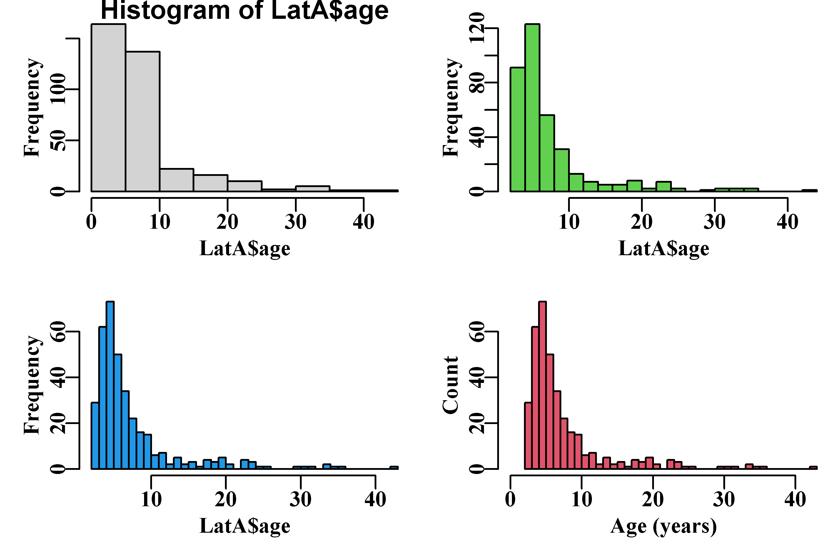
Figure 2.1: An example series of histograms using data from the MQMF data set LatA, illustrating how one can iterate towards a final plot. See also the function uphist().
2.2.9 Dealing with Factors
One aspect of R that can cause frustration and difficulties is the use of factors to represent categorical variables. These convert the categorical variable into levels (the different values) of a factor, even factors that already have numerical values. It is common, for example, to use at least some categorical variables when standardizing fisheries CPUE, thus, if one has depth categories from 50 – 600 m in steps of 50, these need to be treated in the standardization as fixed categorical factors rather than numeric values. But once converted to a set of factors they no longer behave as the original numerical variables, which is generally what is wanted when being plotted. However, if originally they were numeric, they can be recovered using, the function facttonum(). In the example code that explores some issues relating to factors, note the use of the function try() (see also tryCatch()). This is used to prevent the r-code stopping due to the error of trying to multiple a factor by a scalar. This is useful when developing code and when writing books using bookdown and Rmarkdown.
#  [1] 300 350 400 450 500 550 600 300 350 400 450 500 550 600
# Levels: 300 350 400 450 500 550 600# [1] NA# [1] 1 2 3 4 5 6 7 1 2 3 4 5 6 7# [1] 300 350 400 450 500 550 600DepCat <- as.numeric(levels(DepCat))[DepCat] # try ?facttonum
#converts replicates in DepCat to numbers, not just the levels
5 * DepCat[3] # now treat DepCat as numeric # [1] 2000# [1] 300 350 400 450 500 550 600 300 350 400 450 500 550 600
# Levels: 300 350 400 450 500 550 600# [1] 300 350 400 450 500 550 600 300 350 400 450 500 550 600It can often be simpler to take a copy of a data.frame and factorize variables within that copy so that if you want to do further manipulations or plotting using the original variables you do not need to convert them back and forth from numbers to factors.
When data is read into a data.frame within R the default behaviour is to treat strings or characters as factors. You can discover the default settings for very many R options by typing options() into the console. If you search for $stringsAsFactors (note the capitals) you will find it defaults to TRUE. Should you wish to turn this off it can be done easily using options(stringsAsFactors=FALSE). As is obvious from the code chunk on factors some care is needed when working with categorical variables.
2.2.10 Inputting Data
As with all programming languages (and statistical packages) a common requirement is to input one’s data ready for analysis. R is very good at data manipulation and such things are well described in books like Crawley (2007). Of course, there are also many R packages that deal with data manipulation as well. A particularly useful one is dplr, which is part of the tidyverse group. but here we will merely be mentioning a few ways of getting data into R. A very common and low level approach is simply to use text files as an input. I still often use comma-separated-value (.csv) files as being simple to produce and able to be opened and edited from very many different editors. One can use read.csv() or read.table() with very little trouble. Once data has been read into R it can then be saved into more efficiently stored formats by save(object,file="filename.RData"), after which it can be loaded back into R using load(file="filename.RData"). Check out ?save and ?load for details.
In the examples for this book, we will be using data-sets that are part of the MQMF package, but, by copying the formats used in those data-sets, you will be able to use your own data once you have it loaded into R.
2.3 Writing Functions
If you are going to use R to conduct any analyses you will typically type your R code using a text editor and at very least save those scripts for later use. There will be many situations where you will want to repeat a series of commands perhaps with somewhat different input values for the variables and or parameters used. Such situations, and many others, are best served by converting your code into a function, though it is not impossible to use source() as an intermediary step. You will see many examples of functions in the following text and in the MQMF package, and to make full use of the ideas expressed in the text you will find it helpful to learn how to write your own functions.
The structure of a function is always the same:
 #Outline of a function's structure
functionname <- function(argument1, fun,...) {
  # body of the function
  #
  # the input arguments and body of a function can include other
  # functions, which may have their own arguments, which is what
  # the ... is for. One can include other inputs that are used but
  # not defined early on and may depend on what function is brought
  # into the main function. See for example negLL(), and others
  answer <- fun(argument1) + 2
  return(answer)
} # end of functionname
functionname(c(1,2,3,4,5),mean)  # = mean(1,2,3,4,5)= 3 + 2 = 5
# [1] 5We will develop an example to illustrate putting together such functions.
2.3.1 Simple Functions
Very often one might have a simple formula such as a growth function or a function describing the maturity ogive of a fish species. The von Bertalanffy curve, for example, is used rather a lot in fisheries work.
\[\begin{equation} \hat{L_t}=L_{\infty}{\left (1-e^{-K(t-t_0)} \right )} \tag{2.1} \end{equation}\]
This equation can be rendered in R in multiple ways, the first as simple code within a code chunk which steps through the ages in a loop, or is vectorized, or more sensibly, uses the equation translated into a function that can be called multiple times rather than copying the explicit line of code.
 # Implement the von Bertalanffy curve in multiple ways
ages <- 1:20
nages <- length(ages)
Linf <- 50;  K <- 0.2;  t0 <- -0.75
 # first try a for loop to calculate length for each age
loopLt <- numeric(nages)
for (ag in ages) loopLt[ag] <- Linf * (1 - exp(-K * (ag - t0)))
 # the equations are automatically vectorized so more efficient
vecLt <- Linf * (1 - exp(-K * (ages - t0))) # or we can convert
 # the equation into a function and use it again and again
vB <- function(pars,inages) { # requires pars=c(Linf,K,t0)
  return(pars[1] * (1 - exp(-pars[2] * (inages - pars[3]))))
}
funLt <- vB(c(Linf,K,t0),ages)
ans <- cbind(ages,funLt,vecLt,loopLt) | ages | funLt | vecLt | loopLt | ages | funLt | vecLt | loopLt | ages | funLt | vecLt | loopLt |
|---|---|---|---|---|---|---|---|---|---|---|---|
| 1 | 14.766 | 14.766 | 14.766 | 8 | 41.311 | 41.311 | 41.311 | 15 | 47.857 | 47.857 | 47.857 |
| 2 | 21.153 | 21.153 | 21.153 | 9 | 42.886 | 42.886 | 42.886 | 16 | 48.246 | 48.246 | 48.246 |
| 3 | 26.382 | 26.382 | 26.382 | 10 | 44.176 | 44.176 | 44.176 | 17 | 48.564 | 48.564 | 48.564 |
| 4 | 30.663 | 30.663 | 30.663 | 11 | 45.232 | 45.232 | 45.232 | 18 | 48.824 | 48.824 | 48.824 |
| 5 | 34.168 | 34.168 | 34.168 | 12 | 46.096 | 46.096 | 46.096 | 19 | 49.037 | 49.037 | 49.037 |
| 6 | 37.038 | 37.038 | 37.038 | 13 | 46.804 | 46.804 | 46.804 | 20 | 49.212 | 49.212 | 49.212 |
| 7 | 39.388 | 39.388 | 39.388 | 14 | 47.383 | 47.383 | 47.383 |
The use of vectorization makes for much more efficient code than when using a loop, and once one is used to the idea the code also becomes more readable. Of course one could just copy across the vectorized line of R that does the calculation, vecLt <- Linf * (1 - exp(-K * (ages - t0))), instead of using a function call. But one could also include error checking and other details into the function and using a function call should aid in avoiding the accidental introduction of errors. In addition, many functions contain a large number of lines of code so using the function call also makes the whole program more readable and easier to maintain.
 #A vB function with some error checking
vB <- function(pars,inages) { # requires pars=c(Linf,K,t0)
  if (is.numeric(pars) & is.numeric(inages)) {
    Lt <- pars[1] * (1 - exp(-pars[2] * (inages - pars[3])))
  } else { stop(cat("Not all input values are numeric! \n")) }
  return(Lt)
}
param <- c(50, 0.2,"-0.75")
funLt <- vB(as.numeric(param),ages) #try without the as.numeric
halftable(cbind(ages,funLt))
# ages funLt ages funLt
# 1 1 14.76560 11 45.23154
# 2 2 21.15251 12 46.09592
# 3 3 26.38167 13 46.80361
# 4 4 30.66295 14 47.38301
# 5 5 34.16816 15 47.85739
# 6 6 37.03799 16 48.24578
# 7 7 39.38760 17 48.56377
# 8 8 41.31130 18 48.82411
# 9 9 42.88630 19 49.03726
# 10 10 44.17579 20 49.211782.3.2 Function Input Values
Using functions has many advantages. Each function has its own analytical environment and a major advantage is that each function’s environment is insulated from analyses that occur outside of the function. In addition, the global environment, in which much of the work gets done, is isolated from the workings within different functions. Thus, within a function you could declare a variable popnum and changes its values in many ways, but this would have no effect on a variable of the same name outside of the function. This implies that the scope of operations within a function is restricted to that function. There are ways available for allowing what occurs inside a function to directly affect variables outside but rather than teach people bad habits I will only give the hint to search out the symbol ->>. Forgetting the exceptional circumstances, the only way a function should interact with the environment within which it finds itself (one can have functions, within functions, within functions,…) is through its arguments or parameters and through what it returns when complete. In the vB() function we defined just above, the arguments are pars and inages, and it explicitly returns Lt. A function will return the outcome of the last active calculation but in this book we always call return() to ensure what is being returned is explicit and clear. Sometimes one can sacrifice increased brevity for increased clarity.
When using a function one can use its argument names explicitly, vB(pars=param, inages=1:20), or implicitly vB(param,1:20). If used implicitly then the order in which the arguments are entered matters. The function will happily use the first three values of 1:20 as the parameters and treat param=c(50,0.02,-0.75) as the required ages if they are entered in the wrong order (from vB(ages, param) one dutifully obtains the following predicted lengths: 1.0000 -269.4264 -1807.0424). If the argument names are used then the order does not matter. It may feel like more effort to type out all those names but it does make programming easier in the end and acts like yet another source of self-documentation. Of course, one should develop a programming style that suits oneself, and, naturally, one learns from making mistakes.
Software is, by its nature, obedient. If we feed the vB() function its arguments back to front, as we saw, it will still do its best to return an answer or fail trying. With relatively simple software and functions it is not too hard to ensure that any such parameter and data inputs are presented to the functions in the right order and in recognizable forms. Once we start generating more inter-linked and complex software where the output of one process forms the input to others then the planning involved needs to extend to the formats in which arguments and data are used. Error checking then becomes far more important than when just using single functions.
2.3.3 R Objects
We are treating R as a programming language and when writing any software one should take its design seriously. Focussing solely on R there are two principles that assist with such designing (Chambers, 2016, p4).
Everything that exists in R is an object.
Everything that happens in R is a function call.
This implies that every argument or parameter and data set that are input to any function is an R object, just as whatever is returned from a function (if anything) is an R object.
2.3.4 Scoping of Objects
You may have wondered why I used the name inages instead of ages in the vB() function arguments above. This is purely to avoid confusion over the scope of each variable. As mentioned above, in R all operations occur within environments, with the global environment being that which is entered when using the console or a simple script. It is important to realize that any function you write has its own environment which contains the scope of the internal variables. While it is true that even if an R object is not passed to a function as an argument that object can still be seen within a function. However, workings internal to a function are hidden from the global or calling environment. If you define a variable within a function but use the same name as one outside a function, then it will first search within its own environment when the name is used and use the internally defined version rather than the externally defined version. Nevertheless, it is better practice to mostly use names for objects within functions that differ from those used outside the function.
 # demonstration that the globel environment is 'visible' inside a
 # a function it calls, but the function's environment remains
 # invisible to the global or calling environment
vBscope <- function(pars) { # requires pars=c(Linf,K,t0)
  rhside <- (1 - exp(-pars[2] * (ages - pars[3])))
  Lt <- pars[1] * rhside
  return(Lt)
}
ages <- 1:10; param <- c(50,0.2,-0.75)
vBscope(param)
# [1] 14.76560 21.15251 26.38167 30.66295 34.16816 37.03799 39.38760 41.31130
# [9] 42.88630 44.17579# Error in eval(expr, envir, enclos) : object 'rhside' not found2.3.5 Function Inputs and Outputs
Like most software, R functions invariably have inputs and outputs (though both may be NULL; a function’s brackets may be empty, e.g. parsyn()). When inputting vectors of parameters or matrices of data it is sensible to adopt a standard format and by that I mean set a standard format. That way any function dealing with such data can make assumptions about its format. Ideally, it remains a good idea to make data checks before using any input data but that can be simplified by adhering to any standard format decided upon.
It is important to know and understand the structure of the data being fed into each function because a series of vectors needs to be referenced differently to a matrix, which behaves differently to a data.frame. It is usually best to reference a matrix explicitly by its column names as there are no guarantees that all such data-sets will be in the order found in schaef. We can compare schaef[,2] with schaef[,"catch"], with schaef$catch.
| year | catch | effort | cpue | year | catch | effort | cpue |
|---|---|---|---|---|---|---|---|
| 1934 | 60913 | 5879 | 10.3611 | 1945 | 89194 | 9377 | 9.5120 |
| 1935 | 72294 | 6295 | 11.4844 | 1946 | 129701 | 13958 | 9.2922 |
| 1936 | 78353 | 6771 | 11.5719 | 1947 | 160134 | 20381 | 7.8570 |
| 1937 | 91522 | 8233 | 11.1165 | 1948 | 200340 | 23984 | 8.3531 |
| 1938 | 78288 | 6830 | 11.4624 | 1949 | 192458 | 23013 | 8.3630 |
| 1939 | 110417 | 10488 | 10.5279 | 1950 | 224810 | 31856 | 7.0571 |
| 1940 | 114590 | 10801 | 10.6092 | 1951 | 183685 | 18726 | 9.8091 |
| 1941 | 76841 | 9584 | 8.0176 | 1952 | 192234 | 31529 | 6.0971 |
| 1942 | 41965 | 5961 | 7.0399 | 1953 | 138918 | 36423 | 3.8140 |
| 1943 | 50058 | 5930 | 8.4415 | 1954 | 138623 | 24995 | 5.5460 |
| 1944 | 64094 | 6397 | 10.0194 | 1955 | 140581 | 17806 | 7.8951 |
 #examine the properties of the data-set schaef
class(schaef)
a <- schaef[1:5,2]
b <- schaef[1:5,"catch"]
c <- schaef$catch[1:5]
cbind(a,b,c)
mschaef <- as.matrix(schaef)
mschaef[1:5,"catch"]  # ok
d <- try(mschaef$catch[1:5]) #invalid for matrices
d  # had we not used try()eveerything would have stopped.
# [1] "data.frame"
# a b c
# [1,] 60913 60913 60913
# [2,] 72294 72294 72294
# [3,] 78353 78353 78353
# [4,] 91522 91522 91522
# [5,] 78288 78288 78288
# 1934 1935 1936 1937 1938
# 60913 72294 78353 91522 78288
# Error in mschaef$catch : $ operator is invalid for atomic vectors
# [1] "Error in mschaef$catch : $ operator is invalid for atomic vectors\n"
# attr(,"class")
# [1] "try-error"
# attr(,"condition")
# <simpleError in mschaef$catch: $ operator is invalid for atomic vectors>By testing the class of the schaef object we could see it is a data.frame and not a matrix. So handling such inputs may not be as simple as they might appear at first sight. Yes, the order of the columns may change but the names might be different too. So it is up to us to at least make some checks and work to make our software at least partly foolproof. Often we are the only people to use the software we write, but I have found this does not mean I do not need to try to make it foolproof (it seems that sometimes I am foolish).
Notice with schaef that we are using all lowercase column headings, which is not always common. As we have seen, column names are important because it is often better to reference a data.frame as if it were a matrix. Typically, when programming, there are usually more than one option we can use. We could coerce an input data matrix into becoming a data.frame, but we can also force the column names to be lowercase. I know the column names are already lowercase, but here we are talking about a function receiving any given data set.
 #Convert column names of a data.frame or matrix to lowercase
dolittle <- function(indat) {
   indat1 <- as.data.frame(indat)
   colnames(indat) <- tolower(colnames(indat))
   return(list(dfdata=indat1,indat=as.matrix(indat)))
} # return the original and the new version
colnames(schaef) <- toupper(colnames(schaef))
out <- dolittle(schaef)
str(out, width=63, strict.width="cut")
# List of 2
# $ dfdata:'data.frame': 22 obs. of 4 variables:
# ..$ YEAR : int [1:22] 1934 1935 1936 1937 1938 1939 1940 1..
# ..$ CATCH : int [1:22] 60913 72294 78353 91522 78288 110417..
# ..$ EFFORT: int [1:22] 5879 6295 6771 8233 6830 10488 10801..
# ..$ CPUE : num [1:22] 10.4 11.5 11.6 11.1 11.5 ...
# $ indat : num [1:22, 1:4] 1934 1935 1936 1937 1938 ...
# ..- attr(*, "dimnames")=List of 2
# .. ..$ : chr [1:22] "1934" "1935" "1936" "1937" ...
# .. ..$ : chr [1:4] "year" "catch" "effort" "cpue"So, in what follows we will try to only use lowercase column names for our fishery dependent data, we will use standard names “year”, “catch”, “cpue”, etc., but we will also include a statement to convert tolower in our functions where we expect to input data matrices. Such details become more important when inputting more complex list objects containing data matrices of fishery dependent data, age-composition data, vectors of biological constants related to growth, maturity, recruitment, and selectivity, as well as other data besides. Deciding on a standard format and checking such inputs should always be included in the design of any somewhat more complex software.
In the case of schaef, this was data that was used with a surplus production model in an assessment. It is a reasonable idea to develop functions to pre-check a data-set for whether it contains all the required data, whether there are gaps in the data, and other details, before it is used in an assessment One could even develop S3 classes for specific analyses, which would allow one to add functions to generic functions like print, plot, and summary, as well as create new generic method functions of ones own.
Alternatively, it is simple to write functions to generate customizable plots for specific analyses to conduct particular tasks that are likely to be repeated many times. An example can be found with the function plotspmdat(), which will take typical fisheries data and plot up the time-series of catches and of cpue.
 #Could have used an S3 plot method had we defined a class   Fig.2.2
plotspmdat(schaef) # examine the code as an eg of a custom plot 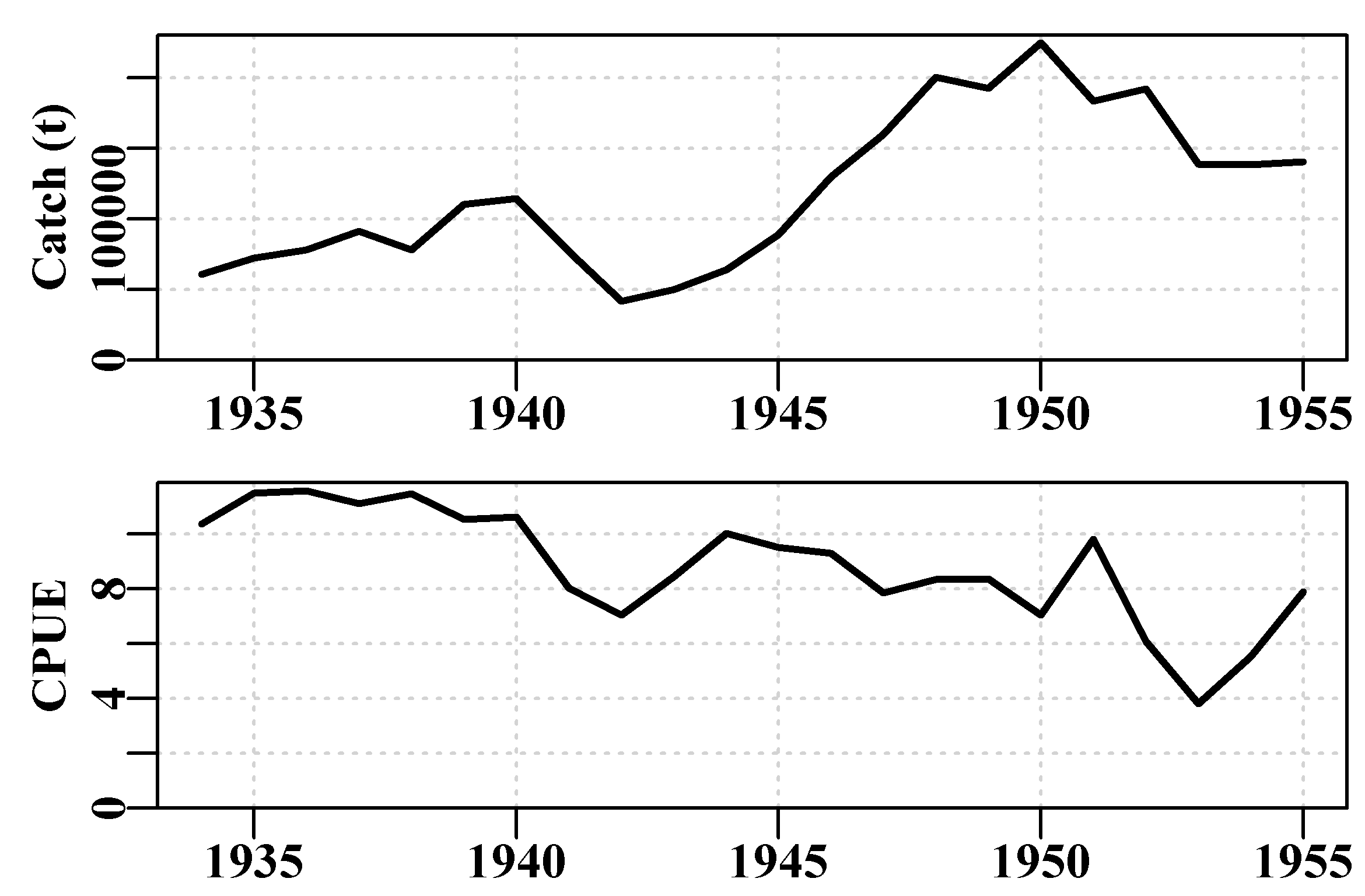
Figure 2.2: The catch and cpue data from the MQMF data-set schaef plotted automatically.
2.4 Appendix: Less-Traveled Functions
The following functions are listed merely to assist the reader in remembering some of the functions within R that tends to be easily forgotten because they are less often used, even though they are very useful when working on real problems.
getNamespaceExports("MQMF")
getS3method("print","default") often print.default works as well
ls(“package:MQMF”) lists the exported functions in the package
ls.str(“package:MQMF”) lists the functions and their syntax
methods(“print”) what S3 methods are available
on.exit(suppressWarnings(sink())) a tidy way to exit a run (even if it fails)
packageDescription("MQMF")
RNGkind() what random number generator is being used
sessionInfo()
sink("filename",split=TRUE) then after lots of screen output sink(),
suppressWarnings(sink()) removes a sink quietly if a run crashes and leaves one open
2.5 Appendix: Additional Learning Resources
Other Books: these two have a tidyverse bent.
Wickham and Grolemund (2017) R for Data Science https://r4ds.had.co.nz/
Grolemund (2014) Hands-On Programming with R https://rstudio-education.github.io/hopr/
There are blogs devoted to R. I rather like https://www.r-bloggers.com/ but I get that delivered to my email. This blog lists many others.
There is even an open-source journal concerning R