Chapter 4 Model Parameter Estimation
4.1 Introduction
One of the more important aspects of modelling in ecology and fisheries science relates to the fitting of models to data. Such model fitting requires:
data from a process of interest in nature (samples, observations),
explicitly selecting a model structure suitable for the task in hand (model design and then selection - big subjects in themselves),
explicitly selecting probability density functions to represent the expected distribution of how predictions of the modelled process will differ from observations from nature when compared (choosing residual error structures), and finally,
searching for the model parameters that optimize the match between the predictions of the model and any observed data (the criterion of model fit).
Much of the skill/trickery/magic that is involved when fitting models to data centers on that innocent looking word or concept optimize in the last requirement above. This is an almost mischievous idea that can occasionally lead one into trouble, though it is also a challenge and can often be fun. The different ways of generating a so-called best-fitting model is an important focus for this chapter. It centers around the idea of what criterion to use when describing the quality of model fit to the available data and how then to implement the explicitly selected criteria.
I keep using the term “explicit”, and for good reason, but some clarification is needed. Very many people will have experienced fitting linear regressions to data but, I am guessing from experience, far fewer people realize that when they fit such a model they are assuming the use of additive normal random residual errors (normal errors) and that they are minimizing the sum of the square of those residuals. In terms of the four requirements above, when applying a linear regression to a data set, the assumption of a linear relationship answers the second requirement, the use of normal errors (with the additional assumption of a constant variance), answers the third requirement, and the minimization of the sum-of squares is the choice that meets the fourth requirement. As is generally the case, it is better to understand explicitly what one is doing rather than just operating out of habit or copying others. In order to make the most appropriate choice of these model fitting requirements (i.e. make selections that can be defended), an analyst also needs an understanding of the natural process being modelled. One can assume and assert almost anything but only so long as such selections can be defended validly. As a more general statement, if one cannot defend a set of choices then one should not make them.
4.1.1 Optimization
In Microsoft Excel, when fitting models to data, the optimum model parameters are found using the built-in Excel Solver. This involves setting up a spreadsheet so that the criterion of optimum fit (sum-of-squares, maximum likelihood, etc, see below) is represented by the contents of a single cell, and the model parameters and data used were contained in other inter-related cells. Altering a model’s parameters would alter the predicted values generated, and this in turn would alter the value of the criterion of optimum fit. A ‘best’ parameter set can be found by searching for the parameters that optimize the match between the observed and the predicted values. It sounds straightforward but turns out to be quite an art form with many assumptions and decisions to be made along the way. In the Excel Solver, one identified the cells containing the model parameters and the Solver’s internal code would then modify those values while monitoring the “criterion of best fit” cell until either a minimum (or maximum) value was found (or an exception was encountered). Effectively such a spreadsheet set-up constitutes the syntax for using the Solver within Excel. We will be using solver or optimization functions in R and they too have a required syntax, but it is no more complex than setting up a spreadsheet, it is just rather more abstract.
Model fitting is usually relatively straightforward when modelling a non-dynamic process to a single set of data, such as length-at-age, with perhaps just two to six parameters. However, it can become much more involved when perhaps dealing with a population’s dynamics through time involving recruitment, the growth of individuals, natural mortality, and fishing mortality from multiple fishing fleets. There may be many types of data, and possibly many 10’s or even 100’s of parameters. In such circumstances, to adjust the quality of the fit of predicted values to observed values some form of automated optimization or non-linear solver is a necessity.
Optimization is a very large subject of study and the very many options available are discussed at length in the CRAN Task View: Optimization and Mathematical Programming found at https://cran.r-project.org/. In the work here, we will mainly use the built-in function nlm() (try ?nlm) but there are many alternatives (including nlminb(), optim(), and others). If you are going to be involved in model fitting it is really worthwhile reading the Task View on optimization on R-CRAN and, as a first step, explore the help and examples given for the nlm() and the optim() functions.
It is sometimes possible to guess a set of parameters that generate what appears to be a reasonable visual fit to the available data, at least for simple static models. However, while such fitting-by-eye may provide usable starting points for estimating a model’s parameters it does not constitute a defensible criterion for fitting models to data. This is so because my fitting-by-eye (or wild-stab-in-the-dark) may well differ from your fitting-by-eye (or educated-guess). Instead of using such opinions some more formally defined criteria of quality of model fit to data is required.
The focus here will be on how to set-up R code to enable model parameter estimation using either least squares or maximum likelihood, especially the latter. Our later consideration of Bayesian methods will be focussed primarily on the characterization of uncertainty. We will illustrate the model fitting process through repeated examples and associated explanations. The objective is that reading this section should enable the reader to set up their own models to solve for the parameter values. We will attempt to do this in a general way that should be amenable to adaptation for many problems.
4.2 Criteria of Best Fit
There are three common options for determining what constitutes an optimum model fit to data.
In general terms, model fitting can involve the minimization of the sum of squared residuals (ssq()) between the values of the observed variable \(x\) and those predicted by candidate models proposed to describe the modelled process, \(\hat{x}\):
\[\begin{equation} ssq=\sum\limits_{i=1}^{n}{({x_i}-{\hat{x}_{i}}}{{)}^{2}} \tag{4.1} \end{equation}\]
where \(x_i\) is observation i from n observations and \({\hat{x}_{i}}\) is the model predicted value for a given observation i (for example, if \(x_i\) was the length-at-age for fish \(i\), then the \({\hat{x}_{i}}\) would be the predicted length-at-age for fish \(i\) derived from some candidate growth model). The use of the \(\hat{}\) in \(\hat{x}\) indicates a predicted value of \(x\).
Alternatively, model fitting can involve minimizing the negative log-likelihood (in this book -veLL or negLL), which entails determining how likely each observed data point is given 1) a defined model structure, 2) a set of model parameters, and 3) the expected probability distribution of the residuals. Minimizing the negative log-likelihood is equivalent to maximizing either the product of all likelihoods or the sum of all log-likelihoods for the set of data points. Given a collection of observations x, a model structure that can predict \(\hat{x}\), and a set of model parameters \(\theta\), then the total likelihood of those observations is defined as:
\[\begin{equation} \begin{split} {L} &= \prod\limits_{i=1}^{n}{{L}\left( {x_i|\theta}\right )} \\ {-veLL} &= -\sum\limits_{i=1}^{n}{ \log{({L}\left( {x_i|\theta}\right )})} \end{split} \tag{4.2} \end{equation}\]
where \(L\) is the total likelihood which is \(\prod{{L}\left( {x|\theta}\right )}\) or the product of the probability density (likelihood) for each observation of \(x\) given the parameter values in \(\theta\) (the further from the expected value in each case, \({\hat{x}_{i}}\), the lower the likelihood). \(-veLL\) is the total negative log-likelihood of the observations \(x\) given the candidate model parameters in \(\theta\), which is the negative sum of the n individual log-likelihoods for each data point in \(x\). We use log-likelihoods because most likelihoods are very small numbers, which when multiplied by many other very small numbers can become so small as to risk leading to floating-point overflow computer errors. Log-transformations change multiplications into additions and avoid such risks (the capital pi, \(\Pi\) turns into a capital sigma, \(\Sigma\)).
A third alternative is to use Bayesian methods that use prior probabilities, which are the initial relative weights given to each of the alternative parameter vectors being considered in the model fitting. Bayesian methods combine with and update any prior knowledge of the most likely model parameters (the prior probabilities) with the likelihoods of any new data that become available given the different candidate parameter vectors \(\theta\). The two key difference between Bayesian methods and maximum likelihood methods, for our purposes, is the inclusion of prior likelihoods and the re-scaling of values so that the posterior probabilities sum to a total of 1.0. An important point is that the likelihood of the data given a set of parameters is being converted into a true probability of the parameters given the data. The posterior probability of a particular parameter set \(\theta\) given the data \(x\) is thus defined as:
\[\begin{equation} P(\theta|x)=\frac{L(x|\theta)P(\theta)}{\sum\limits_{i=1}^{n}{\left[ L(x_i|\theta)P(\theta)\right]}} \tag{4.3} \end{equation}\]
where \({P \left (\theta \right)}\) is the prior probability of the parameter set \(\theta\), which is updated by the likelihood of the data, \(x\), given the parameters, \(\theta\), \(L(x|\theta)P(\theta)\), and the divisor \({\sum\limits_{i=1}^{n}{\left[ L\left (x|\theta \right ) P\left(\theta\right)\right]}}\) re-scales or normalizes the result so the sum of the posterior probabilities for all parameter vectors given the data, \(\sum{P(\theta|x)}\), sums to 1.0. Formally, Equ(4.3) is an approximation as the summation in the divisor should actually be an integration across a continuous distribution, but in practice the approximation suffices and is the only practical option when dealing with the parameters of a complex fisheries model whose Posterior distribution has no simple analytical solution.
Here we will focus mainly on minimizing negative log-likelihoods (equivalent to the maximum likelihood). Although the other methods will also be given some attention. The Bayesian methods will receive much more attention when we explore the characterization of uncertainty.
Microsoft Excel is excellent software for many uses but implementing both maximum likelihood and particularly Bayesian methods tends to be slow and clumsy, they are much more amenable to implementation in R.
Identifying the sum-of-squared residuals, maximum likelihood, and Bayesian methods is not an exhaustive list of the criteria it is possible to use when fitting models to data. For example, it is possible to use the ‘sum of absolute residuals’ (SAR) which avoids the problem of combining positive and negative residuals by using their absolute values rather than squaring them (Birkes and Dodge, 1993). Despite the existence of such alternative criteria of optimal model fit we will focus our attention only on the three mentioned. Other more commonly used alternatives include what are known as robustified methods, which work to reduce the effect of outliers, or extreme and assumed to be atypical values, in available data. As stated earlier, optimization is a large and detailed field of study, I commend it to you for study, and good luck with it.
4.3 Model Fitting in R
While a grid search covering the parameter space might be a possible approach to searching for an optimum parameter set it would become more and more unwieldy as the number of parameters increased above two until eventually it would became unworkable. We will not consider that possibility any further. Instead, to facilitate the search for an optimum parameter set, a non-linear optimizer implemented in software is required.
The R system has a selection of different optimization functions, each using a different algorithm (do see the CRAN task view on Optimization). The solver function (nlm()), like the others, needs to be given an initial guess at the parameter values and then those initial parameter values are varied by the optimizer function and at each change the predicted values are recalculated as in the ssq() or negLL(). Optimization functions, such as nlm(), continue to vary the parameter values (how they do this is where the algorithms vary) until a combination is found that is defined to be the ‘best fit’ according to whatever criterion has been selected (or further improvements cannot be found). Fisheries stock assessment models can often have numerous parameters in the order of 10s or 100s (some have many more and require more highly specialized software e.g. Fournier et al, 1998; Fournier et al, 2012; Kristensen et al, 2016). In this book we will not be estimating large numbers of parameters, but the principles remain similar no matter the number.
4.3.1 Model Requirements
Discussing the theory of model fitting is helpful but does not clarify how one would implement fitting a model in R in practice. The optimizing software is used to vary the values within a parameter vector but we need to provide it with the means of repeatedly calculating the predicted values that will be used to compare with the observed values as many times as required to find the optimum solution (if successful). We need to develop chunks of code that can be repeatedly called, which is exactly the purpose for which R functions are designed. To implement model fitting to real world problems within R we need to consider the four formal requirements:
observations (data) from the system under study. This may be a fishery with observed catches, cpue, age- and length-composition of catches, etc., or it may be something simpler such as the observed lengths and associated ages for a sample of fish (but how to get this into R?),
an R function representing a candidate model of the system that when provided with a vector of parameters is used to calculate predicted values for comparison with whatever observed values are available,
an R function calculating the selected criterion of best fit, the minimum least-squares or minimum negative log-likelihood, to enable a comparison of the observed with the predicted values. This needs to be able to return a single value, reflecting the input parameters and data, that can then be minimized by the final required function, which is
an R function (we will tend to use
nlm()) for automatically optimizing the value of the selected criterion of best fit.
Thus, input data and three functions are needed Figure(4.1) but, because we can use built-in functions to conduct the optimization, model fitting usually entails writing at most two functions, one to calculate the predicted values from whatever model one is using and the other to calculate the criterion of fit (sometimes, in simpler exercises, these two can be combined into one function).
We assume in this book that the reader is at least acquainted with the concepts behind model fitting, as in fitting a linear regression, so we will move straight to non-linear model fitting. The primary aim of these relatively simple examples will be to introduce the use and syntax of the available solvers within R.
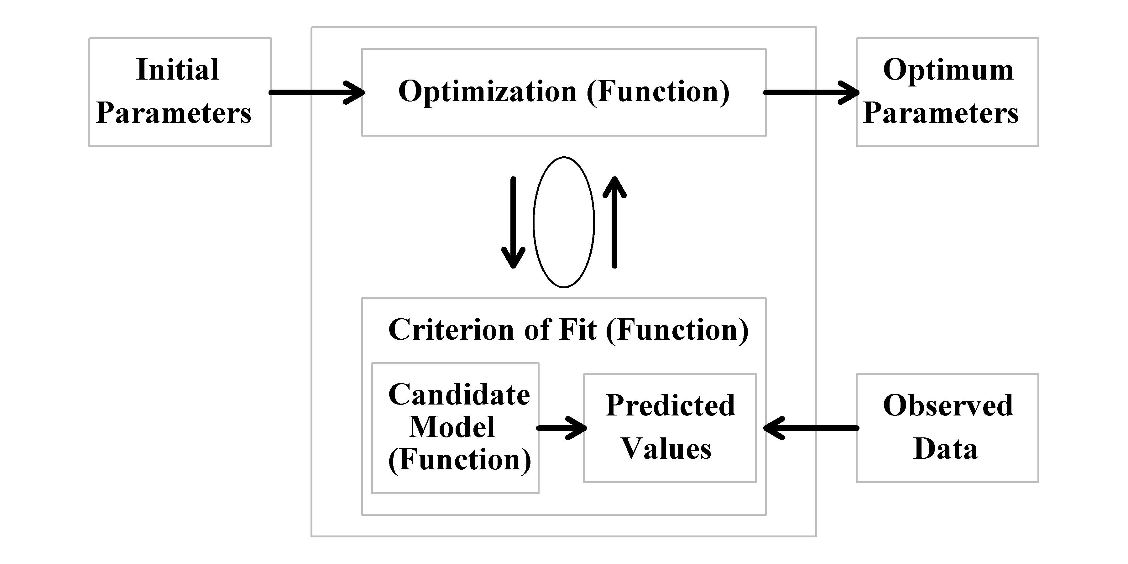
Figure 4.1: Inputs, functional requirements, and outputs, when fitting a model to data. The optimization function (here nlm()) minimizes the negative log-likelihood (or sum-of squares) and requires an initial parameter vector to begin. In addition, the optimizer requires a function (perhaps negLL()) to calculate the corresponding negative log-likelihood for each vector of parameters it produces in its search for the minimum. To calculate the negative log-likelihood requires a function (perhaps vB()) to generate predicted values for comparison with the input observed values.
4.3.2 A Length-at-Age Example
Fitting a model to data simply means estimating the model’s parameters so that its predictions match the observations as well as it can according to the criterion of best-fit chosen. As a first illustration of fitting a model to data in R we will use a simple example of fitting the well-known von Bertalanffy growth curve (von Bertalanffy, 1938), to a set of length-at-age data. Such a data set is included in the R package MQMF (try ?LatA). To use you own data one option is to produce a comma separated variable (csv) file with a minimum of columns of ages and lengths each with a column name (LatA has columns of just age and length; see its help page). Such csv files can be read into R using laa <- read.csv(file="filename.csv", header=TRUE).
The von Bertalanffy length-at-age growth curve is described by:
\[\begin{equation} \begin{split} & {{\hat{L}}_t}={L_{\infty}}\left( 1-{e^{\left( -K\left( t-{t_0} \right) \right)}} \right) \\ & {L_t}={L_{\infty}}\left( 1-{e^{\left( -K\left( t-{t_0} \right) \right)}} \right)+\varepsilon \\ & {L_t}= {\hat{L}}_t + \varepsilon \end{split} \tag{4.4} \end{equation}\]
where \({\hat{L}_t}\) is the expected or predicted length-at-age \(t\), \({L_\infty}\) (pronounced L-infinity) is the asymptotic average maximum body size, \(K\) is the growth rate coefficient that determines how quickly the maximum is attained, and \(t_0\) is the hypothetical age at which the species has zero length (von Bertalanffy, 1938). This non-linear equation provides a means of predicting length-at-age for different ages once we have estimates (or assumed values) for \({L_\infty}\), \(K\), and \(t_0\). When we are fitting models to data we use either of the the bottom two equations in Equ(4.4), where the \(L_t\) are the observed values and these are equated to the predicted values plus a normal random deviate \(\varepsilon = N(0,\sigma^2)\), each value of which could be negative or positive (the observed value can be larger or smaller than the predicted length for a given age). The bottom equation is really all about deciding what residual errors structure to use. In this chapter we will describe an array of alternative error structures used in ecology and fisheries. Not all of them are additive and some are defined using functional relationships rather than constants (such as \(\sigma\)).
The statement about Equ(4.4) being non-linear was made explicitly because earlier approaches to estimating parameter values for the von Bertalanffy (vB()) growth curve involved various transformations that aimed approximately to linearize the curve (e.g. Beverton and Holt, 1957). Fitting the von Bertalanffy curve was no minor undertaking in the late 1950s and 1960s. Happily, such transformations are no longer required, and such curve fitting has become straightforward.
4.3.3 Alternative Models of Growth
There is a huge literature on the study of individual growth and many different models are used to describe the growth of organisms (Schnute and Richards, 1990). The von Bertalanffy (vB()) curve has dominated fisheries models since Beverton and Holt (1957) introduced it more widely to fisheries scientists. However, just because it is very commonly used does not necessarily mean it will always provide the best description of growth for all species. Model selection is a vital if often neglected aspect of fisheries modelling (Burnham and Anderson, 2002; Helidoniotis and Haddon, 2013). Two alternative possibilities to the vB() for use here are the Gompertz growth curve (Gompertz, 1925):
\[\begin{equation} {{\hat{L}}_{t}}=a{{e}^{-b{{e}^{ct}}}}\text{ or }{{\hat{L}}_{t}}=a \exp (-b \exp (ct)) \tag{4.5} \end{equation}\]
and the generalized Michaelis-Menten equation (Maynard Smith and Slatkin, 1973; Legendre and Legendre, 1998):
\[\begin{equation} {{\hat{L}}_{t}}=\frac{at}{b+{{t}^{c}}} \tag{4.6} \end{equation}\]
each of which also have three parameters a, b, and c, and each can provide a convincing description of empirical data from growth processes. Biological interpretations (e.g. maximum average length) can be given to some of the parameters but in the end these models provide only an empirical description of the growth process. If the models are interpreted as reflecting reality this can lead to completely implausible predictions such as non-existent meters-long fish (Knight, 1968). In the literature the parameters can have different symbols (for example, Maynard Smith and Slatkin (1973), use R0 instead of a for the Michaelis-Menton ) but the underlying structural form remains the same. After fitting the von Bertalanffy growth curve to the fish in MQMF’s length-at-age data set LatA, we can use these different models to illustrate the value of trying such alternatives and maintaining an open mind with regard to which model one should use. This issue will arise again when we discuss uncertainty because we can get different results from different models. Model selection is one of the big decisions to be made when modelling any natural process. Importantly, trying different models in this way will also reinforce the processes involved when fitting models to data.
4.4 Sum of Squared Residual Deviations
The classical method for fitting models to data is known as ‘least sum of squared residuals’ (see Equs(4.1) and (4.7)), or more commonly ‘least-squares’ or ‘least-squared’. The method has been attributed to Gauss (Nievergelt, 2000, refers to a translation of Gauss’ 1823 book written in Latin: Theoria combinationis observationum erroribus minimis obnoxiae). Whatever the case, the least-squares approach fits into a strategy used for more than two centuries for defining the best fit of a set of predicted values to those observed. This strategy is to identify a so-called objective function (our criterion of best-fit) which can either be minimized or maximized depending on how the function is structured. In the case of the sum-of-squared residuals one subtracts each predicted value from its associated observed value, square the separate results (to avoid negative values), sum all the values and use mathematics (the analytical solution) or some other approach to minimize that summation:
\[\begin{equation} ssq=\sum\limits_{i=1}^{n}{{{\left( {{O}_{i}}-{\hat{E}_{i}} \right)}^{2}}} \tag{4.7} \end{equation}\]
where, \(ssq\) is the sum-of-squared residuals of \(n\) observations, \(O_i\) is observation \(i\), and \(\hat{E}_i\) is the expected or predicted value for observation \(i\). The function ssq() within MQMF is merely a wrapper surrounding a call to whatever function is used to generate the predicted values and then calculates and returns the sum-of-squared deviations. It is common that we will have to create new functions as wrappers for different problems depending on their complexity and data inputs. ssq() illustrates nicely the fact that in among the arguments that one might pass to a function it is also possible to pass other functions (in this case, within ssq(), we have called the passed a function to funk, but of course when using ssq() we input the actual function relating to the problem at hand, perhaps vB, note with no brackets when used as a function argument).
4.4.1 Assumptions of Least-Squares
A major assumption of least squares methodology is that the residual error terms exhibit a Normal distribution about the predicted variable with equal variance for all values of the observed variable; that is, in the \(\varepsilon=N(0,\sigma^2)\) the \(\sigma^2\) is a constant. If data are transformed in any way, the transformation effects on the residuals may violate this assumption. Conversely, a transformation may standardize the residual variances if they vary in a systematic way. Thus, if data are log-normally distributed then a log-transformation will normalize the data and least squares can then be used validly. As always, a consideration or visualization of the form of both the data and the residuals, resulting from fitting a model, is good practice.
4.4.2 Numerical Solutions
Most of the interesting problems in fisheries science do not have an analytical solution (e.g. as available for linear regression) and it is necessary to use numerical methods to search for an optimum model fit using a defined criterion of “best fit”, such as the minimum sum of squared residuals (least-squares). This will obviously involve a little R programming, but a big advantage of R is that once you have a set of analyses developed it can become straightforward to apply them to a new set of data.
In the examples below we use some of the utility functions from MQMF to help with the plotting. But for fitting and comparing the three different growth models defined above we need five functions, four of which we need to write. The first three are used to estimate the predicted values of length-at-age used to compare with the observed data. This example has three alternative model functions, vB(), Gz(), and mm(), one each for the three different growth curves. The fourth function is needed to calculate the sum-of-squared residuals from the predicted values and their related observations. Here we are going to be using the MQMF function ssq() (whose code you should examine and understand). This function returns a single value which is to be minimized by the final function, nlm(), which is needed to do the minimization in an automated manner. The R function nlm(), uses a user-defined generalized function, that it refers to as f (try args(nlm), or formals(nlm) to see the full list of arguments), for calculating the minimum (in this case of ssq()), which, in turn, uses the function defined for predicted lengths-at-age from the growth curve (e.g. vB()). Had we used a different growth curve function (e.g. Gz()) we only have to change everywhere the nlm() calling code points to vB() to Gz() and modify the parameter values to suit the Gz() function for the code to produce a usable result. Fundamentally, nlm() minimizes ssq() by varying the input parameters (which it refers to as p) that alter the outcome of the growth function vB(), Gz(), or mm(), whichever is selected.
nlm() is just one of the functions available in R for conducting non-linear optimization, alternatives include optim() and nlminb() (do read the documentation in ?nlm, and the task view on optimization on CRAN lists packages aimed at solving optimization problems).
 #setup optimization using growth and ssq
data(LatA)      # try ?LatA   assumes library(MQMF) already run
 #convert equations 4.4 to 4.6 into vectorized R functions
 #These will over-write the same functions in the MQMF package
vB <- function(p, ages) return(p[1]*(1-exp(-p[2]*(ages-p[3]))))
Gz <- function(p, ages) return(p[1]*exp(-p[2]*exp(p[3]*ages)))
mm <- function(p, ages) return((p[1]*ages)/(p[2] + ages^p[3]))
 #specific function to calc ssq. The ssq within MQMF is more
ssq <- function(p,funk,agedata,observed) {        #general and is
  predval <- funk(p,agedata)        #not limited to p and agedata
  return(sum((observed - predval)^2,na.rm=TRUE))
} #end of ssq
 # guess starting values for Linf, K, and t0, names not needed
pars <- c("Linf"=27.0,"K"=0.15,"t0"=-2.0) #ssq should=1478.449
ssq(p=pars, funk=vB, agedata=LatA$age, observed=LatA$length)
# [1] 1478.449The ssq() function replaces the MQMF::ssq() function in the global environment, but it also returns a single number, e.g. the 1478.449 above, which is the first input to the nlm() function and is what gets minimized.
4.4.3 Passing Functions as Arguments to other Functions
In the last example we defined some of the functions required to fit a model to data. We defined the growth models we were going to compare and we defined a function to calculate the sum-of-squares. A really important aspect of what we just did was that to calculate the sum-of-squares we passed the vB() function as an argument to the ssq() function. What that means is that we have passed a function that has arguments as one of the arguments to another function. You can see the potential for confusion here so it is necessary to concentrate and keep things clear. Currently, the way we have defined ssq() this all does not seem so remarkable because we have explicitly defined the arguments to both functions in the call to ssq(). But R has some tricks up its sleeve that we can use to generalize such functions that contain other functions as arguments and the main one uses the magic of the ellipsis .... With any R function, unless an argument has a default value set in its definition, each argument must be given a value. In the ssq() function above we have included both the arguments used only by ssq() (funk and observed), and those used only by the function funk (p and agedata). This works well for the example because we have deliberately defined the growth functions to have identical input arguments but what if the funk we wanted to use had different inputs, perhaps because we were fitting a selectivity curve and not a growth curve? Obviously we would need to write a different ssq() function. To allow for more generally useful functions that can be re-used in many more situations, the writers of R (R Core Team, 2019) included this concept of ..., which will match any arguments not otherwise matched, and so can be used to input the arguments of the funk function. So, we could re-define ssq() thus:
 # Illustrates use of names within function arguments
vB <- function(p,ages) return(p[1]*(1-exp(-p[2] *(ages-p[3]))))
ssq <- function(funk,observed,...) { # only define ssq arguments
  predval <- funk(...) # funks arguments are implicit
  return(sum((observed - predval)^2,na.rm=TRUE))
} # end of ssq
pars <- c("Linf"=27.0,"K"=0.15,"t0"=-2.0) # ssq should = 1478.449
ssq(p=pars, funk=vB, ages=LatA$age, observed=LatA$length) #if no
ssq(vB,LatA$length,pars,LatA$age) # name order is now vital!
# [1] 1478.449
# [1] 1478.449This means the ssq() function is now much more general and can be used with any input function that can be used to generate a set of predicted values for comparison with a set of observed values. This is how the ssq() function within MQMF is implemented; read the help ?ssq. The general idea is that you must define all arguments used within the main function but any arguments only used within the called function (here called funk), can be passed in the …. It is always best to explicitly name the arguments so that their order does not matter, and you need to be very careful with typing as if you misspell the name of an argument passed through the … this will not always throw an error! For example, using a uppercase LatA$Age rather than LatA$age does not throw an error but leads to a result of zero rather than 1478.440. This is because LatA$Age = NULL, which is a valid if incorrect input. Clearly the … can be very useful but it is also inherently risky if you type as badly as I do.
 # Illustrate a problem with calling a function in a function
 # LatA$age is typed as LatA$Age but no error, and result = 0
ssq(funk=vB, observed=LatA$length, p=pars, ages=LatA$Age) # !!!
# [1] 0And if you were rushed and did not bother naming the arguments that too will fail if you get the arguments out of order. If, for example, you were to input ssq(LatA$length, vB, pars, LatA$age) instead of ssq(vB, LatA$length, pars, LatA$age) then you will get an error: Error in funk(…) : could not find function “funk”. You might try that yourself just to be sure. It rarely hurts to experiment with your code, you cannot break your computer and you might learn something.
4.4.4 Fitting the Models
If we plot up the LatA data set Figure(4.2), we see some typical length-at-age data. There are 358 points (try dim(LatA)) and many lie on top of each other, but the relative sparseness of fish in the older age classes becomes apparent when we use the rgb() option within the plot() function to vary the transparency of colour in the plot. Alternatively, we could use jitter() to add noise to each plotted point’s position to see the relative density of data points. Whenever you are dealing with empirical data it is invariably worth your time to at least plot it up and otherwise explore its properties.
 #plot the LatA data set   Figure 4.2
parset()        # parset and getmax are two MQMF functions
ymax <- getmax(LatA$length) # simplifies use of base graphics. For
 # full colour, with the rgb as set-up below, there must be >= 5 obs
plot(LatA$age,LatA$length,type="p",pch=16,cex=1.2,xlab="Age Years",
     ylab="Length cm",col=rgb(1,0,0,1/5),ylim=c(0,ymax),yaxs="i",
xlim=c(0,44),panel.first=grid()) 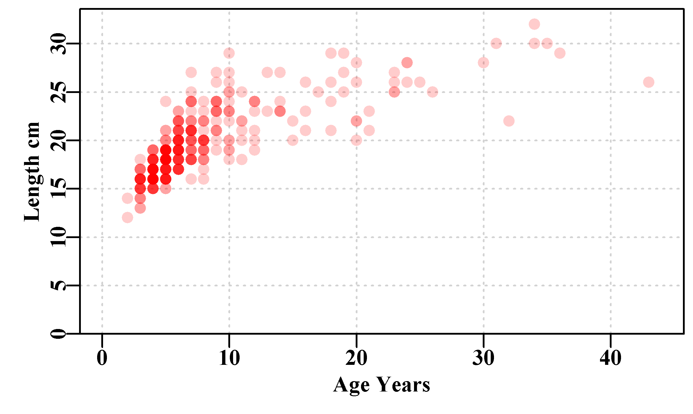
Figure 4.2: Simulated female length-at-age data for 358 Redfish, Centroberyx affinis, based on samples from eastern Australia. Full intensity colour means >= 5 points.
Rather than continuing to guess parameter values and modifying them by hand we can use nlm() (or optim(), or nlminb(), which have different syntax for their use) to fit growth models or curves to the selected LatA data. This will illustrate the syntax of nlm() but also the use of two more MQMF utility R functions magnitude() and outfit() (check out ?nlm, ?magnitude, and ?outfit). You might also look at the code in each function (enter each function’s name into the console without arguments or brackets). From now on I will prompt you less often to check out the details of functions that get used, but if you see a function that is new to you hopefully, by now, it makes sense to review its help, its syntax, and especially its code, just as you might look at the contents of each variable that gets used.
Each of the three growth models require the estimation of three parameters and we need initial guesses for each to start off the nlm() solver. All we do is provide values for each of the nlm() function’s parameters/arguments. In addition, we have used two extra arguments, typsize and iterlim. The typsize is defined in the nlm() help as “an estimate of the size of each parameter at the minimum”. Including this often helps to stabilize the searching algorithm used as it works to ensure that the iterative changes made to each parameter value are of about the same scale. A very common alternative approach, which we will use with more complex models, is to log-transform each parameter when input into nlm() and back-transform them inside the function called to calculate the predicted values. However, this could only work where the parameters are guaranteed to always stay positive. With the von Bertalanffy curve, for example, the \(t_0\) parameter is often negative and so magnitude() should be used instead of the log-transformation strategy. The default iterlim=100 means a maximum of 100 iterations, which is sometimes not enough, so if 100 are reached you should expand this number to, say, 1000. You will quickly notice that the only thing changed between each model fitting effort is the function that funk, inside ssq(), is pointed at and the starting parameter values. This is possible by consciously designing the growth functions to use exactly the same arguments (passed via …). You could also try running one or two of these without setting the typsize and interlim options. Notice also that we have run the Michaelis-Menton curve with two slightly different starting points.
 # use nlm to fit 3 growth curves to LatA, only p and funk change
ages <- 1:max(LatA$age) # used in comparisons
pars <- c(27.0,0.15,-2.0) # von Bertalanffy
bestvB <- nlm(f=ssq,funk=vB,observed=LatA$length,p=pars,
             ages=LatA$age,typsize=magnitude(pars))
outfit(bestvB,backtran=FALSE,title="vB"); cat("\n")
pars <- c(26.0,0.7,-0.5) # Gompertz
bestGz <- nlm(f=ssq,funk=Gz,observed=LatA$length,p=pars,
             ages=LatA$age,typsize=magnitude(pars))
outfit(bestGz,backtran=FALSE,title="Gz"); cat("\n")
pars <- c(26.2,1.0,1.0) # Michaelis-Menton - first start point
bestMM1 <- nlm(f=ssq,funk=mm,observed=LatA$length,p=pars,
             ages=LatA$age,typsize=magnitude(pars))
outfit(bestMM1,backtran=FALSE,title="MM"); cat("\n")
pars <- c(23.0,1.0,1.0) # Michaelis-Menton - second start point
bestMM2 <- nlm(f=ssq,funk=mm,observed=LatA$length,p=pars,
             ages=LatA$age,typsize=magnitude(pars))
outfit(bestMM2,backtran=FALSE,title="MM2"); cat("\n")
# nlm solution: vB
# minimum : 1361.421
# iterations : 24
# code : 2 >1 iterates in tolerance, probably solution
# par gradient
# 1 26.8353971 -1.133838e-04
# 2 0.1301587 -6.195068e-03
# 3 -3.5866989 8.326176e-05
#
# nlm solution: Gz
# minimum : 1374.36
# iterations : 28
# code : 1 gradient close to 0, probably solution
# par gradient
# 1 26.4444554 2.724757e-05
# 2 0.8682518 -6.455226e-04
# 3 -0.1635476 -2.046463e-03
#
# nlm solution: MM
# minimum : 1335.961
# iterations : 12
# code : 2 >1 iterates in tolerance, probably solution
# par gradient
# 1 20.6633224 -0.02622723
# 2 1.4035207 -0.37744316
# 3 0.9018319 -0.05039283
#
# nlm solution: MM2
# minimum : 1335.957
# iterations : 25
# code : 1 gradient close to 0, probably solution
# par gradient
# 1 20.7464274 8.465730e-06
# 2 1.4183164 -3.856475e-05
# 3 0.9029899 -1.297406e-04These are numerical solutions and they do not guarantee a correct solution. Notice that the gradients in the first Michaelis-Menton solution (that started at 26.2, 1, 1) are relatively large and yet it’s SSQ, at 1335.96, is very close to the second Michaelis-Menton model fit and smaller (better) than either the vB or Gz curves. However, the gradient values indicate that this model fit can, and should be, improved. If you alter the initial parameter estimate for parameter a (the first MM parameter) down to 23 instead of 26.2, as in the last model fit, we obtain slightly different parameter values, a slightly smaller SSQ, and much smaller gradients giving greater confidence that the result is a real minimum. As it happens, if one were to run cbind(mm(bestMM1$estimate,ages), mm(bestMM2$estimate,ages)) you can work out that the predicted values differ from -0.018 to 0.21% while, if you include the vB predictions, MM2 differs from the vB predictions from -6.15 to 9.88% (ignoring the very largest deviation of 40.6%). You could also try omitting the typsize argument from the estimate of the vB model, which will still give the optimal result but inspect the gradients to see why using typsize helps the optimization along. When setting up these examples, occasional runs of the Gz() model gave rise to a comment that the steptol might be too small and changing it from the default of 1e-06 to 1e-05 quickly fixed the problem. If it happens to you, add a statement ,steptol=1e-05 to the nlm() command and see if the diagnostics improve.
The obvious conclusion is that one should always read the diagnostic comments from nlm(), consider the gradients of the solution one obtains, and it is always a good idea to use multiple sets of initial parameter guesses to ensure one has a stable solution. Numerical solutions are based around software implementations and the rules used to decide when to stop iterating can sometimes be fooled by sub-optimal solutions. The aim is to find the global minimum not a local minimum. Any non-linear model can give rise to such sub-optimal solutions so automating such model fitting is not a simple task. Never assume that the first answer you get in such circumstances is definitely the optimum you are looking for, even if the plotted model fit looks acceptable.
Within a function call if you name each argument then the order does not strictly matter, but I find that consistent usage simplifies reading the code so would recommend using the standard order even when using explicit names. If we do not use explicit names the syntax for nlm() requires the function to be minimized (f) to be defined first. It also expects the f function, whatever it is, to use the initial parameter guess in the p argument, which, if unnamed must come second. If you type formals(nlm) or args(nlm) into the console one obtains the possible arguments that can be input to the function along with their defaults if they exist:
# function (f, p, ..., hessian = FALSE, typsize = rep(1,
#   length(p)),fscale = 1, print.level = 0, ndigit = 12,
#   gradtol = 1e-06, stepmax = max(1000 *
#   sqrt(sum((p/typsize)^2)), 1000), steptol = 1e-06,
#   iterlim = 100, check.analyticals = TRUE)
As you can see the function to be minimized f (in this case ssq()) comes first, followed by the initial parameters, p, that must be the first argument required by whatever function is pointed to by f. Then comes the ellipsis (three dots) that generalizes the nlm() code for any function f, and then a collection of possible arguments all of which have default values. We altered typsize and iterlim (and steptol in Gz() sometimes); see the nlm() help for an explanation of each.
In R the … effectively means whatever other inputs are required, such as the arguments for whatever function f is pointed at (in this case ssq). If you look at the args or code, or help for ?ssq, you will see that it requires the function, funk, that will be used to calculate the expected values relative to the next required input for ssq(), which is the vector of observed values (as in \(O_i - E_i\)). Notice there is no explicit mention of the arguments used by funk, which are assumed to be passed using the …. In each of our calls to ssq() we have filled in those arguments explicitly with, for example, nlm(f=ssq,funk=Gz, observed=LatA$length, p=pars, ages=LatA$age, ). In that way all the requirements are filled and ssq() can do its work. If you were to accidentally omit, say, the ages=LatA$age, argument then, helpfully (in this instance), R will respond with something like Error in funk(par, independent) : argument “ages” is missing, with no default (I am sure you believe me but it does not hurt to try it for yourself!).
In terms of the growth curve model fitting, plotting the results provides a visual comparison that illustrates the difference between the three growth curves (Murrell, 2011).
 #Female length-at-age + 3 growth fitted curves Figure 4.3
predvB <- vB(bestvB$estimate,ages) #get optimumpredicted lengths
predGz <- Gz(bestGz$estimate,ages) # using the outputs
predmm <- mm(bestMM2$estimate,ages) #from the nlm analysis above
ymax <- getmax(LatA$length) #try ?getmax or getmax [no brackets]
xmax <- getmax(LatA$age)  #there is also a getmin, not used here
parset(font=7)   # or use parsyn() to prompt for the par syntax
plot(LatA$age,LatA$length,type="p",pch=16, col=rgb(1,0,0,1/5),
     cex=1.2,xlim=c(0,xmax),ylim=c(0,ymax),yaxs="i",xlab="Age",
     ylab="Length (cm)",panel.first=grid())
lines(ages,predvB,lwd=2,col=4)        # vB    col=4=blue
lines(ages,predGz,lwd=2,col=1,lty=2)  # Gompertz  1=black
lines(ages,predmm,lwd=2,col=3,lty=3)  # MM        3=green
 #notice the legend function and its syntax.
legend("bottomright",cex=1.2,c("von Bertalanffy","Gompertz",
"Michaelis-Menton"),col=c(4,1,3),lty=c(1,2,3),lwd=3,bty="n") 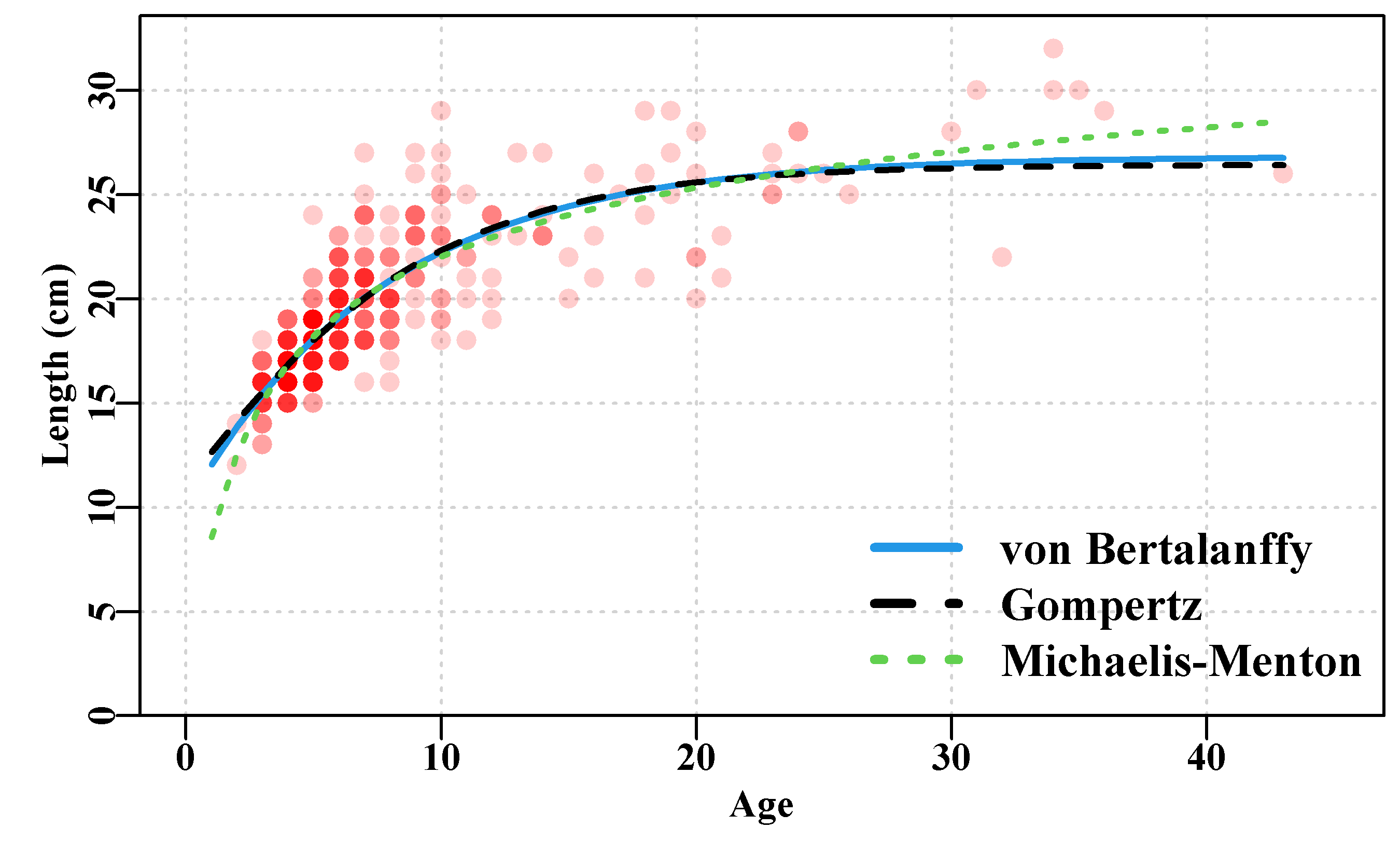
Figure 4.3: Female Length-at-Age data from 358 simulated female redfish with three optimally fitted growth curves drawn on top.
The rgb() function used in the plot implies that the intensity of colour represents the number of observations, with the most intense implying at least five observations. It is clear that with this data the vB() and Gz() curves are close to coincident over much of the extent of the observed data, while the mm() curve deviates from the other two but mainly at the extremes. The Michaelis-Menton curve is forced to pass through the origin, while the other two are not constrained in this way (even though the idea may appear to be closer to reality). One could include the length of post-larval fish to pull the Gompertz and von Bertalanffy curves downwards. But with living animals growth is complex. Many sharks and rays have live-birth and do start post-development life at sizes significantly above zero. Always remember that these curves are empirical descriptions of the data and have limited abilities to reflect reality.
Most of the available data is between ages 3 and 12 (try table(LatA$age)), and then only single occurrences above age 24. Over the ages 3 - 24 the Gompertz and von Bertalanffy curves follow essentially the same trajectory and the Michaelis-Menton curve differs only slightly (you could try the following code to see the actual differences cbind(ages, predvB, predGz, predmm). Outside of that age range bigger differences occur, although the lack of younger animals suggests the selectivity of the gear that caught the samples may under-represent fish less than 3 years old. In terms of the relative quality of fit (the sum-of-squared residuals) the final Michaelis-Menton curve has the smallest ssq(), followed by the von Bertalanffy, followed by the Gompertz. But each provides a plausible mean description of the growth between the range of 3 - 24 years, where the data is most dense. When data is as sparse as it is in the older age classes there is also the question of whether or not this sample is representative of the population for those ages. Questioning one’s data,the model used, and consequent interpretations, is an important aspect of producing useful models of natural processes.
4.4.5 Objective Model Selection
In the three growth models above the optimum model fit was defined as that which minimized the sum-of-squared residuals between the predicted and observed values. By that criterion the second Michaelis-Menton curve provided a ‘better’ fit than either von Bertalanffy or the Gompertz curves. But can we really say that the second Michaelis-Menton curve was ‘better’ fitting than the first? In terms of the gradients of the final solution things are clearly better with the second curve but strictly the criterion of fit was only the minimum SSQ and the difference was less than 0.01 units. Model selection is generally a trade-off between the number of parameters used and the quality of fit according to the criterion chosen. If we devise a model with more parameters this generally leads to greater flexibility and improved capacity to be closer to the observed data. In the extreme if we had as many parameters as we had observations we could have a perfect model fit, but, of course, would have learned nothing about the system we are modelling. With 358 parameters for the LatA data set that would clearly be a case of over-parameterization, but what if we had only increased the number of parameters to say 10? No doubt the curve would have been oddly shaped but would likely have a lower SSQ. Burnham and Anderson (2002) provide a detailed discussion of the trade-off between number of parameters and quality of model fit to data. In the 1970s there was a move to using Information Theory to develop a means of quantifying the trade-off between model parameters and quality of model fit. Akaike (1974) described his Akaike’s Information Criterion (AIC), which was based on maximum likelihood and information theoretic principles (more of which later) but fortunately, Burnham and Anderson (2002) provide an alternative when using the minimum sum-of-squared residuals, which is a variant of one included in Atkinson (1980):
\[\begin{equation} AIC=N \left(log\left(\hat\sigma^2 \right) \right)+2p \tag{4.8} \end{equation}\]
where \(N\) is the number of observations, \(p\) is the “number of independently adjusted parameters within the model” (Akaike, 1974, p716), and \(\hat\sigma^2\) is the maximum likelihood estimate of the variance, which just means the sum-of-squared residuals is divided by \(N\) rather than \(N-1\):
\[\begin{equation} \hat\sigma^2 = \frac{\Sigma\varepsilon^2}{N} = \frac{ssq}{N} \tag{4.9} \end{equation}\]
Even with the \(AIC\) it is difficult to determine, when using least-squares, whether differences can be argued to be statistically significantly different. There are ways related to the analysis of variance but such questions are able to be answered more robustly when using maximum likelihood, so we will address that in a later section.
If one wants to obtain biologically plausible or defensible interpretations when fitting a model, then model selection cannot be solely dependent upon quality of statistical fit. Instead, it should reflect the theoretical expectations (for example, should average growth in a population involve a smooth increase in size through time, etc.). Such considerations, other than statistical fit to data, do not appear to gain sufficient attention, but only become important when biologically implausible model outcomes arise or implausible model structures are proposed. It obviously helps to have an understanding of the biological expectations of the processes being modelled.
4.4.6 The Influence of Residual Error Choice on Model Fit
In the growth model example, we used Normal random deviates, but we can ask the question of whether we would have obtained the same answer had we used, for example, log-normal deviates? All we need to do in that case would be to log-transform the observed and predicted values before calculating the sum-of-squared residuals (see below with reference to log-normal residuals.
\[\begin{equation} ssq=\sum\limits_{i=1}^{n}{{{\left( log({O_i})- log({\hat{E_i}}) \right)}^{2}}} \tag{4.10} \end{equation}\]
Here we continue to use the backtran=FALSE option within outfit() because we are log-transforming the data not the parameters so no back-transformation is required.
 # von Bertalanffy
pars <- c(27.25,0.15,-3.0)
bestvBN <- nlm(f=ssq,funk=vB,observed=LatA$length,p=pars,
             ages=LatA$age,typsize=magnitude(pars),iterlim=1000)
outfit(bestvBN,backtran=FALSE,title="Normal errors"); cat("\n")
 # modify ssq to account for log-normal errors in ssqL
ssqL <- function(funk,observed,...) {
  predval <- funk(...)
  return(sum((log(observed) - log(predval))^2,na.rm=TRUE))
} # end of ssqL
bestvBLN <- nlm(f=ssqL,funk=vB,observed=LatA$length,p=pars,
             ages=LatA$age,typsize=magnitude(pars),iterlim=1000)
outfit(bestvBLN,backtran=FALSE,title="Log-Normal errors")
# nlm solution: Normal errors
# minimum : 1361.421
# iterations : 22
# code : 1 gradient close to 0, probably solution
# par gradient
# 1 26.8353990 -3.649702e-07
# 2 0.1301587 -1.576574e-05
# 3 -3.5867005 3.198205e-07
#
# nlm solution: Log-Normal errors
# minimum : 3.153052
# iterations : 25
# code : 1 gradient close to 0, probably solution
# par gradient
# 1 26.4409587 8.906655e-08
# 2 0.1375784 7.537147e-06
# 3 -3.2946087 -1.124171e-07In this case the curves produced by using normal and log-normal residual errors barely differ Figure(4.4), even though their parameters differ (use ylim=c(10,ymax) to make the differences clearer). More than differing visually, the different model fits are not even comparable. If we compare their respective sum-of-squared residuals one has 1361.0 and the other only 3.153. This is not surprising when we consider the effect of the log-transformations within the calculation of the sum-of-squared. But what this means is we cannot look at the tabulated outputs alone and decide which version fits the data better than the other. They are strictly incommensurate even though they are using exactly the same model. The use of the different residual error structure needs to be defended in ways other than considering the relative model fit. This example emphasizes that while the choice of model is obviously important, the choice of residual error structure is part of the model structure and equally important.
 # Now plot the resultibng two curves and the data Fig 4.4
predvBN <- vB(bestvBN$estimate,ages)
predvBLN <- vB(bestvBLN$estimate,ages)
ymax <- getmax(LatA$length)
xmax <- getmax(LatA$age)
parset()
plot(LatA$age,LatA$length,type="p",pch=16, col=rgb(1,0,0,1/5),
     cex=1.2,xlim=c(0,xmax),ylim=c(0,ymax),yaxs="i",xlab="Age",
     ylab="Length (cm)",panel.first=grid())
lines(ages,predvBN,lwd=2,col=4,lty=2)   # add Normal dashed
lines(ages,predvBLN,lwd=2,col=1)        # add Log-Normal solid
legend("bottomright",c("Normal Errors","Log-Normal Errors"),
col=c(4,1),lty=c(2,1),lwd=3,bty="n",cex=1.2) 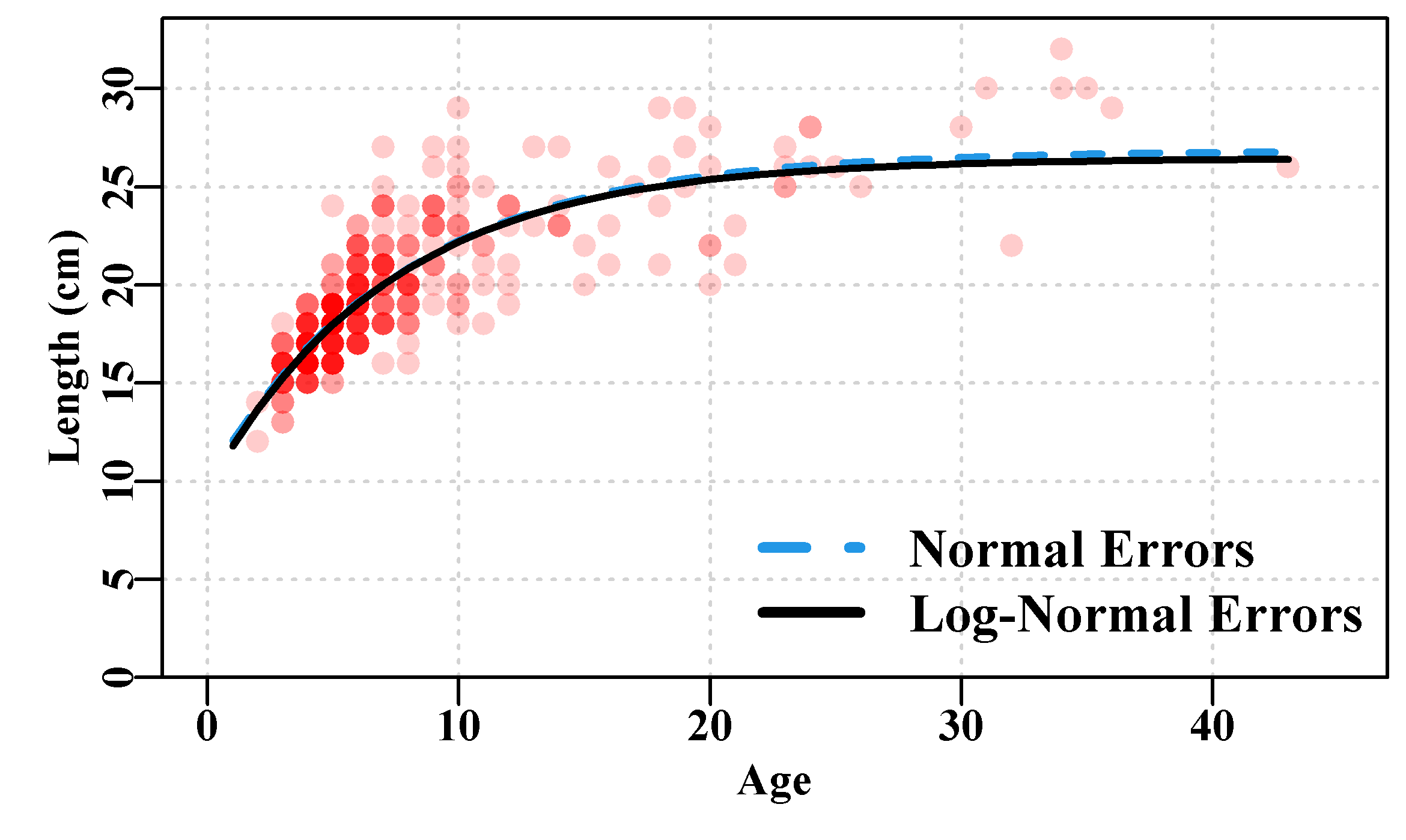
Figure 4.4: Female Length-at-Age data from 358 female redfish, Centroberyx affinis, with two von Bertalanffy growth curves fitted using Normal and Log-Normal residuals.
4.4.7 Remarks on Initial Model Fitting
The comparison of curves in the example above is itself interesting, however, what we have also done is illustrate the syntax of nlm() and how one might go about fitting models to data. The ability to pass functions as arguments into another function (as here we passed ssq as f into nlm(), and vB, Gz, and mm into ssq() as funk) is one of the strengths but also complexities of R. In addition, the use of the … to pass extra arguments without having to name them explicitly beforehand helps produce re-usable code. It simplifies the re-use of functions like ssq() where all we need do is change the input function, with potentially completely different input requirements, to get an entirely different answer from essentially the same code. The very best way of becoming familiar with these methods is to employ them with your own data sets. Plot your data and any model fits because if the model fit appears unusual then it quite likely is, and deserves a second and third look.
One can go a long way using sum-of-squares but the assumptions requiring normally distributed residuals around the expected values, and a constant variance are constraining when dealing with the diversity of the real world. In order to use probability density distributions other than Normal and to use non-constant variances, one should turn to using maximum likelihood.
4.5 Maximum Likelihood
The use of likelihoods is relatively straightforward in R as there are built-in functions for very many Probability Density Functions (PDFs) as well as an array of packages that define other PDFs. To repeat, the aim with maximum likelihood methods is to use software to search for the model parameter set that maximizes the total likelihood of the observations. To use this criterion of optimal model fit requires the model to be defined so that it specifies probabilities or likelihoods for each of the observations (the available data) as a function of the parameter values and other variables within the model (Equ(4.2) and Equ(4.11)). Importantly, such a specification includes an estimate of the variability or spread of the selected PDF (the \(\sigma\) in the Normal distribution; which is only a by-product of the least-squares approach). A major advantage of using maximum likelihood is that the residual structure or the expected distribution of observations about the expected central tendency of the data need not be normally distributed. If the probability density function (PDF) can be defined, it can be used in a maximum likelihood framework; see Forbes et al, (2011) for the definitions of many useful probability density functions.
4.5.1 Introductory Examples
We will use the well-known Normal distribution to illustrate the methods but then extend the approach to include an array of alternative PDFs. For the purposes of model fitting to data the primary interest for each PDF is in the definition of the probability density or likelihood for individual observations. For a Normal distribution with a mean expected value of \({\bar{x}}\) or \({\mu}\), the probability density or likelihood of a given single value \(x_i\) is defined as:
\[\begin{equation} L\left( {x_i}|\mu_{i} ,\sigma \right)=\frac{1}{\sigma \sqrt{2\pi }}{{e}^{\left( \frac{-{{\left( {x_i}-\mu_{i} \right)}^{2}}}{2\sigma^2 } \right)}} \tag{4.11} \end{equation}\]
where \({\sigma}\) is the standard deviation associated with \({\mu_{i}}\). This identifies an immediate difference between least-squared methods and maximum likelihood methods, in the latter, one needs a full definition of the PDF, which in the case of the Normal distribution includes an explicit estimate of the standard deviation of the residuals around the mean estimates \(\mu\). Such an estimate is not required with least-squares, although is easily derived from the SSQ value.
As an example, we can generate a sample of observations from a Normal distribution (see ?rnorm) and then calculate that sample’s mean and stdev and compare how likely the given sample values are for these parameter estimates relative to how likely they are for the original mean and stdev used in the rnorm function, Table(4.1):
 # Illustrate Normal random likelihoods. see Table 4.1
set.seed(12345)       # make the use of random numbers repeatable
x <- rnorm(10,mean=5.0,sd=1.0)      # pseudo-randomly generate 10
avx <- mean(x)                      # normally distributed values
sdx <- sd(x)          # estimate the mean and stdev of the sample
L1 <- dnorm(x,mean=5.0,sd=1.0)   # obtain likelihoods, L1, L2 for
L2 <- dnorm(x,mean=avx,sd=sdx)    # each data point for both sets
result <- cbind(x,L1,L2,"L2gtL1"=(L2>L1))      # which is larger?
result <- rbind(result,c(NA,prod(L1),prod(L2),1)) # result+totals
rownames(result) <- c(1:10,"product")
colnames(result) <- c("x","original","estimated","est > orig") | x | original | estimated | est > orig | |
|---|---|---|---|---|
| 1 | 5.5855 | 0.33609530 | 0.33201297 | 0 |
| 2 | 5.7095 | 0.31017782 | 0.28688183 | 0 |
| 3 | 4.8907 | 0.39656626 | 0.49010171 | 1 |
| 4 | 4.5465 | 0.35995784 | 0.45369729 | 1 |
| 5 | 5.6059 | 0.33204382 | 0.32465621 | 0 |
| 6 | 3.1820 | 0.07642691 | 0.05743702 | 0 |
| 7 | 5.6301 | 0.32711267 | 0.31586172 | 0 |
| 8 | 4.7238 | 0.38401358 | 0.48276941 | 1 |
| 9 | 4.7158 | 0.38315644 | 0.48191389 | 1 |
| 10 | 4.0807 | 0.26144927 | 0.30735328 | 1 |
| product | 0.00000475 | 0.00000892 | 1 |
The bottom line of Table(4.1) contains the product (obtained using the R function prod()) of each of the columns of likelihoods. Not surprisingly the maximum likelihood is obtained when we use the sample estimates of the mean and stdev (estimated, L2) rather than the original values of mean=5 and sd=1.0 (original, L1); that is 8.9201095^{-6} > 4.7521457^{-6}. I can be sure of these values in this example because the set.seed() R function was used at the start of the code to begin the pseudo-random number generators at a specific location. If you commonly use set.seed() do not repeatedly use the same old sequences, such as 12345, as you risk undermining the idea of of the pseudo-random numbers being a good approximation to a random number sequence, perhaps use getseed() to provide a suitable seed number instead.
So rnorm() provides pseudo-random numbers from the distribution defined by the mean and stdev, dnorm() provides the probability density or likelihood of an observation given its mean and stdev (the equivalent of Equ(4.11)). The cumulative probability density function (cdf) is provided by the function pnorm(), and the quantiles are identified by qnorm(). The mean value will naturally have the largest likelihood. Note also that the normal curve is symmetrical around the mean.
 # some examples of pnorm, dnorm, and qnorm, all mean = 0
cat("x = 0.0        Likelihood =",dnorm(0.0,mean=0,sd=1),"\n")
cat("x = 1.95996395 Likelihood =",dnorm(1.95996395,mean=0,sd=1),"\n")
cat("x =-1.95996395 Likelihood =",dnorm(-1.95996395,mean=0,sd=1),"\n")
 # 0.5 = half cumulative distribution
cat("x = 0.0        cdf = ",pnorm(0,mean=0,sd=1),"\n")
cat("x = 0.6744899  cdf = ",pnorm(0.6744899,mean=0,sd=1),"\n")
cat("x = 0.75       Quantile =",qnorm(0.75),"\n") # reverse pnorm
cat("x = 1.95996395 cdf = ",pnorm(1.95996395,mean=0,sd=1),"\n")
cat("x =-1.95996395 cdf = ",pnorm(-1.95996395,mean=0,sd=1),"\n")
cat("x = 0.975      Quantile =",qnorm(0.975),"\n") # expect ~1.96
 # try x <- seq(-5,5,0.2); round(dnorm(x,mean=0.0,sd=1.0),5)
# x = 0.0 Likelihood = 0.3989423
# x = 1.95996395 Likelihood = 0.05844507
# x =-1.95996395 Likelihood = 0.05844507
# x = 0.0 cdf = 0.5
# x = 0.6744899 cdf = 0.75
# x = 0.75 Quantile = 0.6744898
# x = 1.95996395 cdf = 0.975
# x =-1.95996395 cdf = 0.025
# x = 0.975 Quantile = 1.959964As we can see, individual likelihoods can be relatively large numbers, however, when multiplied together they can quickly lead to relatively small numbers. Errors can arise when the number of observations increases. Even with only ten numbers when we multiply all the individual likelihoods together (using prod()) the outcome quickly becomes very small indeed. With another similar ten numbers to the ten used in Table(4.1) the overall likelihood could easily be down to 1e-11 or 1e-12. As the number of observations increases the chances of a rounding error (even on a 64-bit computer) begin to increase. Rather than multiply many small numbers to get an extremely small number the standard solution to multiplying these small numbers together is to natural-log-transform the likelihoods and then add them together. Maximizing the sum of the log-transformed likelihoods obtains the optimum parameters exactly as does maximizing the product of the individual likelihoods. In addition, many optimizers, in software, appear to have been designed to be most efficient at minimizing a function. The simple solution is instead of maximizing the product of the individual likelihoods we minimize the sum of the negative log-likelihoods (-veLL or negLL()).
4.6 Likelihoods from the Normal Distribution
Likelihoods can appear to be rather strange beasts. When from continuous PDFs they are not strictly probabilities although they share many of their properties (Edwards, 1972). Strictly they relate to the probability density at a particular point under a probability density function. The area under the full curve must, by the definition of probabilities, sum to 1.0, but the area under any single point of a continuous PDF becomes infinitesimally small. Normal likelihoods are defined using Equ(4.11)), whereas the cumulative density function is:
\[\begin{equation} {cdf}=1=\int\limits_{x=-\infty }^{\infty }{\frac{1}{\sigma \sqrt{2\pi }}}{{e}^{\left( \frac{-{{\left( x-\mu \right)}^{2}}}{2{{\sigma }^{2}}} \right)}} \tag{4.12} \end{equation}\]
We can use dnorm() and pnorm() to calculate both the likelihoods and the cdf (Figure(4.5)).
 # Density plot and cumulative distribution for Normal   Fig 4.5
x <- seq(-5,5,0.1)  # a sequence of values around a mean of 0.0
NL <- dnorm(x,mean=0,sd=1.0)   # normal likelihoods for each X
CD <- pnorm(x,mean=0,sd=1.0)   # cumulative density vs X
plot1(x,CD,xlab="x = StDev from Mean",ylab="Likelihood and CDF")
lines(x,NL,lwd=3,col=2,lty=3) # dashed line as these are points
abline(h=0.5,col=4,lwd=1) 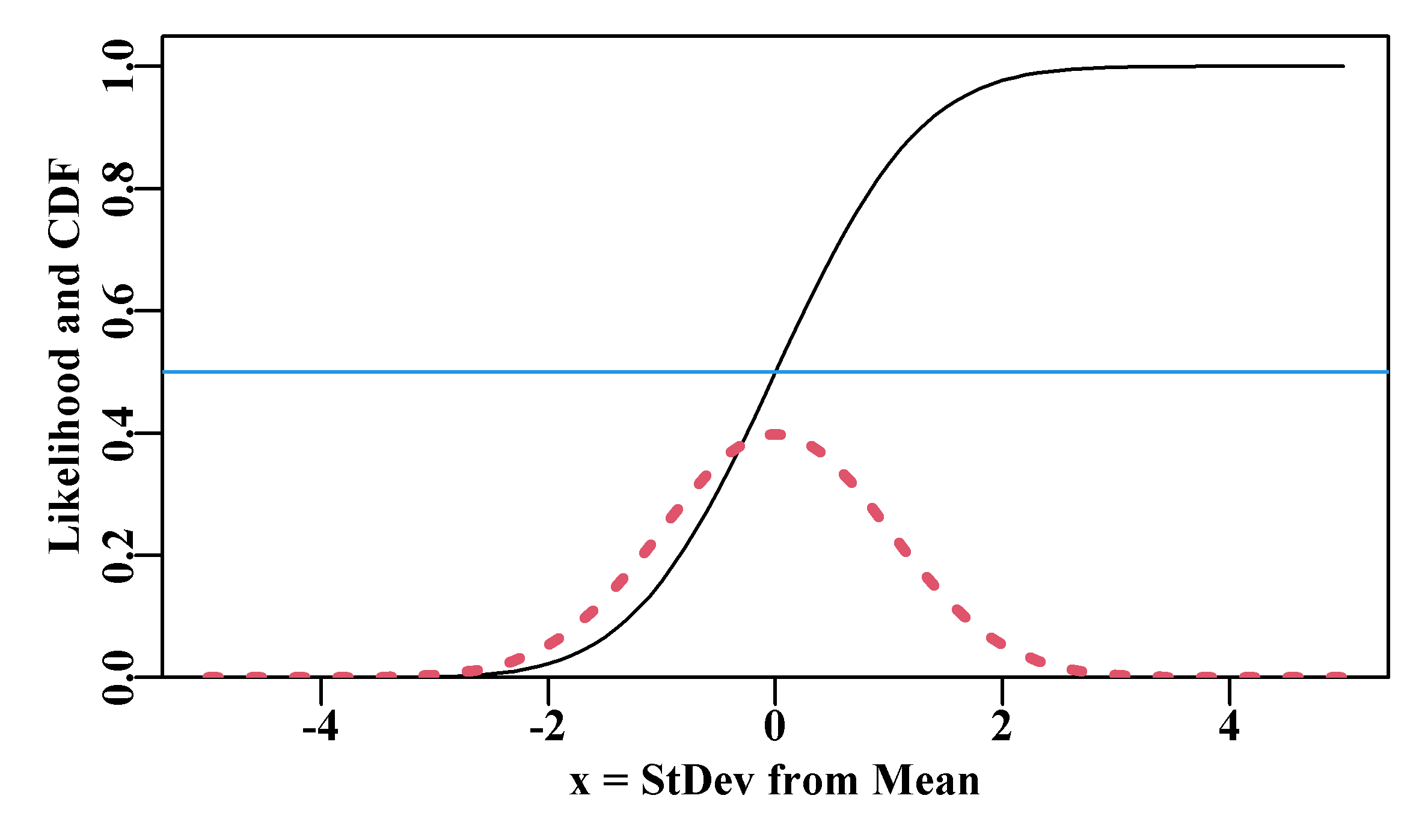
Figure 4.5: A dotted red curve depicting the expected normal likelihoods for a mean = 0 and sd = 1.0, along with the cumulative density of the same normal likelihoods as a black line. The blue line identifies a cumulative probability of 0.5.
That all sounds fine, but what does it mean to identify a specific value under such a curve for a specific value of the \(x\) variable? In Figure(4.5) we used a dotted line to suggest that the likelihoods in the plot are local estimates and do not make up a continuous line. Each represents the likelihood at exactly the given \(x\) value. We have seen above that the probability density at a value of 0.0 for a distribution with mean = 0.0 and stdev = 1.0 would be 0.3989423. Let us briefly examine this potential confusion between likelihood and probability. If we consider a small portion of the probability density function with a mean = 5.0, and st.dev = 1.0 between the values of x = 3.4 to 3.6 we might see something like Figure(4.6):
 #function facilitates exploring different polygons Fig 4.6
plotpoly <- function(mid,delta,av=5.0,stdev=1.0) {
   neg <- mid-delta;  pos <- mid+delta
   pdval <- dnorm(c(mid,neg,pos),mean=av,sd=stdev)
   polygon(c(neg,neg,mid,neg),c(pdval[2],pdval[1],pdval[1],
                          pdval[2]),col=rgb(0.25,0.25,0.25,0.5))
   polygon(c(pos,pos,mid,pos),c(pdval[1],pdval[3],pdval[1],
                                pdval[1]),col=rgb(0,1,0,0.5))
   polygon(c(mid,neg,neg,mid,mid),
        c(0,0,pdval[1],pdval[1],0),lwd=2,lty=1,border=2)
   polygon(c(mid,pos,pos,mid,mid),
        c(0,0,pdval[1],pdval[1],0),lwd=2,lty=1,border=2)
   text(3.395,0.025,paste0("~",round((2*(delta*pdval[1])),7)),
        cex=1.1,pos=4)
   return(2*(delta*pdval[1])) # approx probability, see below
} # end of plotpoly, a temporary function to enable flexibility
 #This code can be re-run with different values for delta
x <- seq(3.4,3.6,0.05) # where under the normal curve to examine
pd <- dnorm(x,mean=5.0,sd=1.0) #prob density for each X value
mid <- mean(x)
delta <- 0.05  # how wide either side of the sample mean to go?
parset()       # a pre-defined MQMF base graphics set-up for par
ymax <- getmax(pd)    # find maximum y value for the plot
plot(x,pd,type="l",xlab="Variable x",ylab="Probability Density",
     ylim=c(0,ymax),yaxs="i",lwd=2,panel.first=grid())
approxprob <- plotpoly(mid,delta) #use function defined above 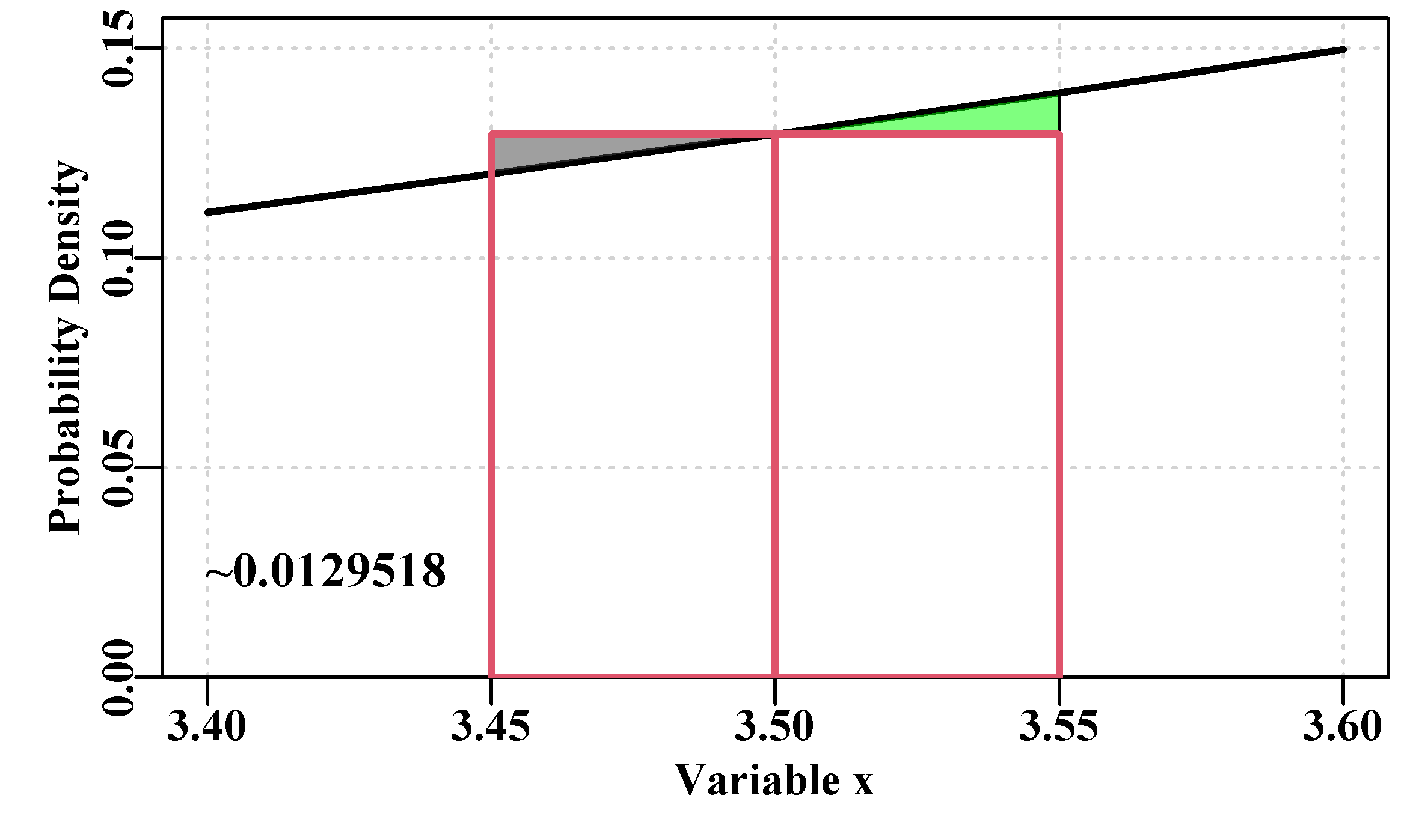
Figure 4.6: Probability densities for a normally distributed variate X, with a mean of 5.0 and a standard deviation of 1.0. The PDF value at x = 3.5 is 0.129518, so the area of the boxes outlined in red is 0.0129518, which approximates the total probability of a value between 3.45 - 3.55, which would really be the area under the curve.
The area under the complete PDF sums to 1.0, so the probability of obtaining a value between, say, 3.45 and 3.55, in Figure(4.6), is the sum of the areas of the oblongs minus the left triangle plus the right triangle. The triangles are almost symmetrical and so approximately cancel each other out, so an approximate solution is simply 2.0 times the area of one of the oblongs. With a delta (width of oblong on x-axis) of 0.05 that probability = 0.0129518. If you change the delta to become 0.01 then the approximate probability = 0.0025904, and as the delta value decreases so does the total probability although the probability density at 3.5 remains the same at 0.1295176. Clearly likelihoods are not identical to probabilities in continuous PDFs (see Edwards, 1972). The best estimate of the probability of the area under the curve is obtained with pnorm(3.55,5,1) - pnorm(3.45,5,1), which = 0.0129585.
4.6.1 Equivalence with Sum-of-Squares
When using normal likelihoods to fit a model to data what we actually do is set things up so as to minimize the sum of the negative log-likelihoods for each available observation. Fortunately, we can use dnorm() to estimate those likelihoods. In fact, if we fit a model using maximum likelihood methods with Normally distributed residuals, or log-transformed Log-Normal distributed data, then the parameter estimates obtained are the same as those obtained using the least-squared approach (see the derivation and form of Equ(4.19), below). Fitting a model would require generating a set of predicted values \({\hat{x}}\) (x-hat) as a function of some other independent variable(s) \(\theta(x)\), where \({\theta}\) is the list of parameters used in the functional relationship. The log-likelihood for \(n\) observations would be defined as:
\[\begin{equation} LL(x|\theta)=\sum\limits_{i=1}^{n}{log\left( \frac{1}{\hat{\sigma }\sqrt{2\pi }}{{e}^{\left( \frac{-{{\left( {x_i}-{{\hat{x}}_{i}} \right)}^{2}}}{2{{{\hat{\sigma }}}^{2}}} \right)}} \right)} \tag{4.13} \end{equation}\]
\(LL(x|\theta)\) is read as the log-likelihood of \(x\), the observations, given \(\theta\) the parameters (\(\mu\) and \(\hat{\sigma}\)); the symbol \(|\) is read as “given”. This superficially complex equation can be greatly simplified. First, we could move the constant before the exponential term outside of the summation term by multiplying it by \(n\), and the natural log of the remaining exponential term back-transforms the exponential:
\[\begin{equation} LL(x|\theta)=n log\left( \frac{1}{\hat{\sigma }\sqrt{2\pi }} \right)+\frac{1}{2{\hat{\sigma }^{2}}}\sum\limits_{i=1}^{n}{\left( -{{\left( x_i-\hat{x}_i \right)}^{2}} \right)} \tag{4.14} \end{equation}\]
The value of \({\hat{\sigma }^{2}}\) is the maximum likelihood estimate of the variance of the data (note the division by \(n\) rather than \(n-1\):
\[\begin{equation} {{\hat{\sigma }}^{2}}=\frac{\sum\limits_{i=1}^{n}{{{\left( x_i-\hat{x}_i \right)}^{2}}}}{n} \tag{4.15} \end{equation}\]
If we replace the use of \({\hat{\sigma }^{2}}\) in Equ(4.14)) with Equ(4.15), the \((x_i-{\hat{x}_i})^2\) cancels out leaving \(-n/2\):
\[\begin{equation} LL(x|\theta)=n{log}\left( \left( {\hat{\sigma }\sqrt{2\pi }} \right)^{-1} \right) - \frac{n}{2} \tag{4.16} \end{equation}\]
simplifying the square root term means bringing the \(-1\) out of the log term, which changes the \(n\) to \(-n\) and we can change the square root to an exponent of 1/2 and add \(\log{(\hat \sigma)}\) to the log of the \(\pi\) term:
\[\begin{equation} LL(x|\theta)=-n\left( {log}\left( {{\left( 2\pi \right)}^{\frac{1}{2}}} \right)+{log}\left( {\hat{\sigma }} \right) \right)-\frac{n}{2} \tag{4.17} \end{equation}\]
then move the power of \(1/2\) to outside the first \(log\) term:
\[\begin{equation} LL(x|\theta)=-\frac{n}{2}\left( {log}\left( 2\pi \right)+2{log}\left( {\hat{\sigma }} \right) \right)-\frac{n}{2} \tag{4.18} \end{equation}\]
then simplify the \(n/2\) and multiply throughout by \(-1\) to convert to a negative log-likelihood to give the final simplification of the negative log-likelihood for normally distributed values:
\[\begin{equation} -LL(x|\theta)=\frac{n}{2}\left( {log}\left( 2\pi \right) + 2{log} \left( {\hat{\sigma }} \right) + 1 \right) \tag{4.19} \end{equation}\]
The only non-constant part of this is the value of \(\hat \sigma\), which is the square root of the sum of squared residuals divided by \(n\), so now it should be clear why the parameters obtained when using maximum likelihood, if using normal random errors, are the same as derived from a least squares approach.
4.6.2 Fitting a Model to Data using Normal Likelihoods
We can repeat the example using the simulated female Redfish data in the data-set LatA, Figure(4.7), which we used to illustrate the use of sum-of-squared residuals. Ideally, we should obtain the same answer but with an estimate of \(\sigma\) as well. The MQMF function plot1() is just a quick way of plotting a single graph (either type=“l” or type=“p”; see ?plot1), without too much white space. Edit plot1() if you like more white space than I do!
 #plot of length-at-age data  Fig 4.7
data(LatA) # load the redfish data set into memory and plot it
ages <- LatA$age;  lengths <- LatA$length
plot1(ages,lengths,xlab="Age",ylab="Length",type="p",cex=0.8,
pch=16,col=rgb(1,0,0,1/5)) 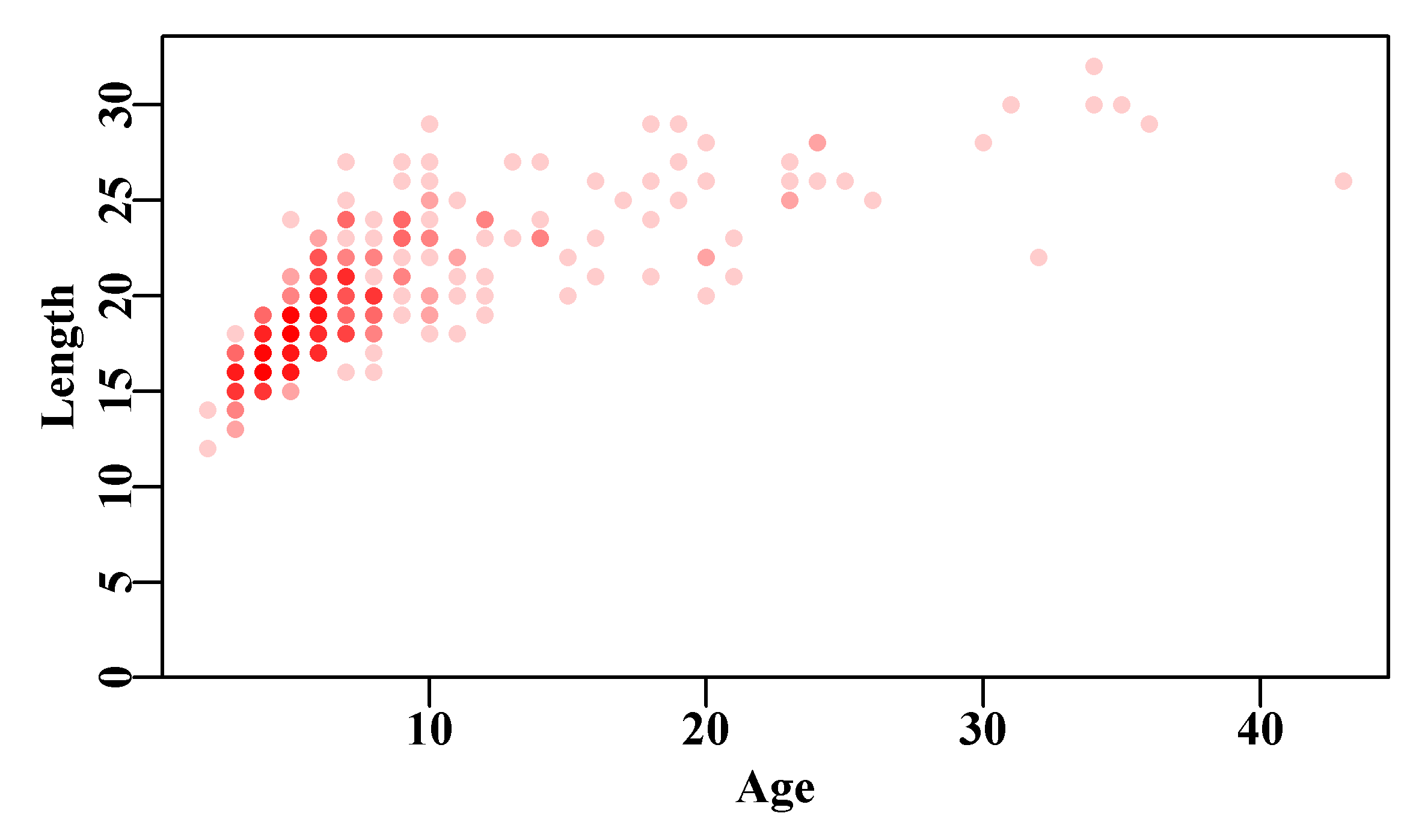
Figure 4.7: The length-at-age data contained within the LatA data set for female Redfish Centroberyx affinis. Full colour means >= 5 points.
Now we can use the MQMF function negNLL() (as in negative normal log-likelihoods) to determine the sum of the negative log-likelihoods using normal random errors (negLL() does the same but for log-normally distributed data). If you look at the code for negNLL() you will see that, just like ssq(), it is passed a function as an argument, which is then used to calculate the predicted mean values for each input age (in this case lengths-at-age using the MQMF function vB()), and then uses dnorm() to calculate the sum of the -veLL using the predicted values as the mean values and the observations of the length-at-age values in the data. The ages data is passed through the ellipsis (…) without being explicitly declared as an argument in negNLL(). The function is very similar in structure to ssq() in that it has identical input requirements, however, pars is passed explicitly rather than inside …, because the last value of pars, must be the stdev of the residuals, which is used inside negNLL() rather than just inside funk. The use of likelihoods means there is a need to include an estimate of the standard deviation at the end of the vector of parameters. negNLL() thus operates in a manner very similar to ssq() in that it is a wrapper for calling the function that generates the predicted values and then uses dnorm() to return a single number every time it is called. Thus, nlm() minimizes negNLL(), which in turn calls vB().
 # Fit the vB growth curve using maximum likelihood
pars <- c(Linf=27.0,K=0.15,t0=-3.0,sigma=2.5) # starting values
 # note, estimate for sigma is required for maximum likelihood
ansvB <- nlm(f=negNLL,p=pars,funk=vB,observed=lengths,ages=ages,
             typsize=magnitude(pars))
outfit(ansvB,backtran=FALSE,title="vB by minimum -veLL")
# nlm solution: vB by minimum -veLL
# minimum : 747.0795
# iterations : 26
# code : 1 gradient close to 0, probably solution
# par gradient
# 1 26.8354474 4.490629e-07
# 2 0.1301554 1.659593e-05
# 3 -3.5868868 3.169513e-07
# 4 1.9500896 8.278354e-06If you look back at the ssq() example for the von Bertalanffy curve, you will see we obtained an SSQ value of 1361.421 from a sample of 358 fish (try nrow(LatA)). Thus the estimate of \(\sigma\) from the ssq() approach was \(\sqrt{ \left (1361.421 / 358 \right)} = 1.95009\), which, as expected, is essentially identical to the maximum likelihood estimate.
Just as before all we need do is substitute a different growth curve function into the negNLL() to get a result. We just have to remember to include a fourth parameter (\(\sigma\)) in the p vector. Once again, using Normal random errors leads to essentially the same numerical solution as that obtained using the ssq() approach.
 #Now fit the Michaelis-Menton curve
pars <- c(a=23.0,b=1.0,c=1.0,sigma=3.0) # Michaelis-Menton
ansMM <- nlm(f=negNLL,p=pars,funk=mm,observed=lengths,ages=ages,
             typsize=magnitude(pars))
outfit(ansMM,backtran=FALSE,title="MM by minimum -veLL")
# nlm solution: MM by minimum -veLL
# minimum : 743.6998
# iterations : 34
# code : 1 gradient close to 0, probably solution
# par gradient
# 1 20.7464280 -6.195465e-06
# 2 1.4183165 1.601881e-05
# 3 0.9029899 2.461405e-04
# 4 1.9317669 -3.359816e-06Once again the gradients of the solution are small, which increases confidence that the solution is not just a local minimum, so we should plot out the solution to see its relative fit to the data.
By plotting the fitted curves on top of the data points the data do not obscure the lines. The actual predictions that can now be produced from this analysis can also be tabulated along with the residual values. By including the individual squared residuals, it becomes more clear which points (see record 3) could have the most influence.
 #plot optimum solutions for vB and mm. Fig 4.8
Age <- 1:max(ages) # used in comparisons
predvB <- vB(ansvB$estimate,Age) #optimum solution
predMM <- mm(ansMM$estimate,Age) #optimum solution
parset()                       # plot the deata points first
plot(ages,lengths,xlab="Age",ylab="Length",type="p",pch=16,
     ylim=c(10,33),panel.first=grid(),col=rgb(1,0,0,1/3))
lines(Age,predvB,lwd=2,col=4)     # then add the growth curves
lines(Age,predMM,lwd=2,col=1,lty=2)
legend("bottomright",c("von Bertalanffy","Michaelis-Menton"),
col=c(4,1),lwd=3,bty="n",cex=1.2,lty=c(1,2)) 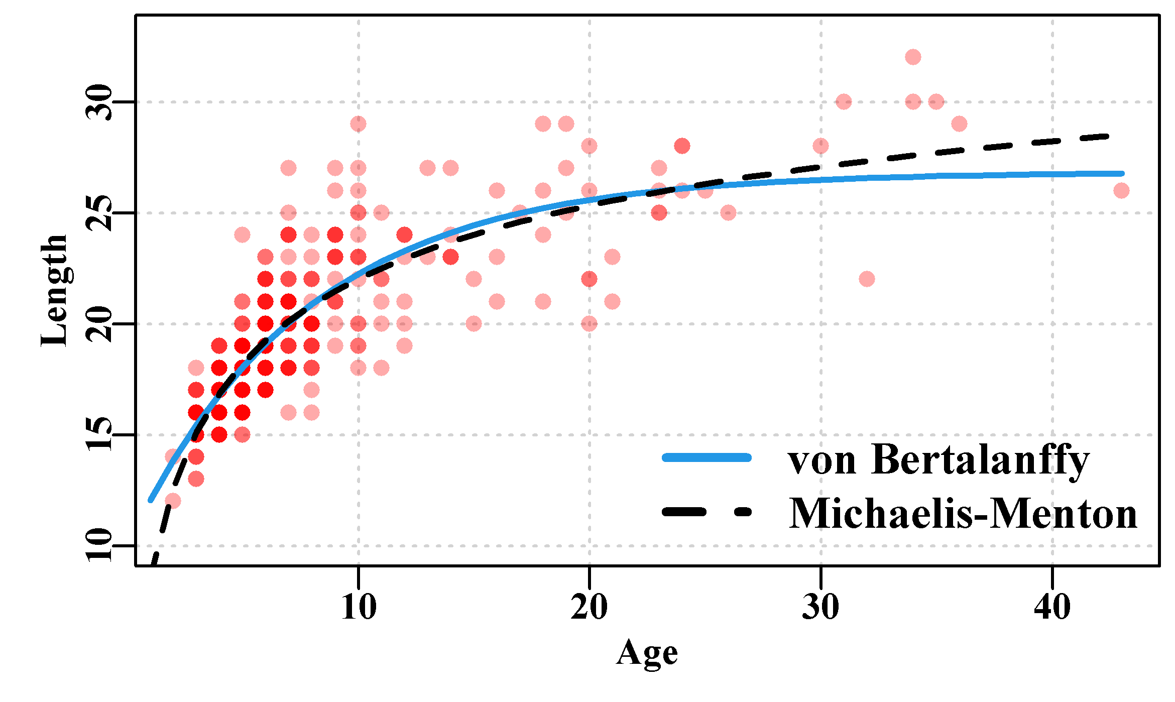
Figure 4.8: Optimum von Bertalanffy and Michaelis-Menton growth curves fitted to the female LatA Redfish data. Note the two curves are effectively coincident where the observations are most concentrated. Note the y-axis starts at 10.
Generally, one would generate residual plots so as to check for patterns in the residuals, Figure(4.9).
 # residual plot for vB curve   Fig 4.9
predvB <- vB(ansvB$estimate,ages) # predicted values for age data
resids <- lengths - predvB               # calculate vB residuals
plot1(ages,resids,type="p",col=rgb(1,0,0,1/3),xlim=c(0,43),
      pch=16,xlab="Ages Years",ylab="Residuals")
abline(h=0.0,col=1,lty=2)    # emphasize the zero line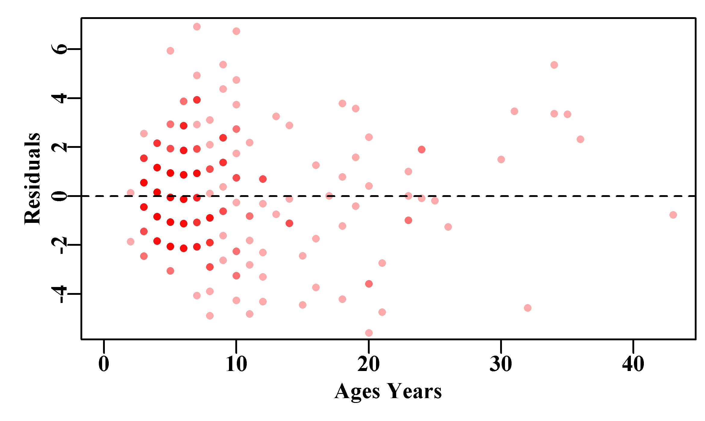
Figure 4.9: The residual values for von Bertalanffy curve fitted to the female LatA data. There is a clear pattern between the ages of 3 - 10, which reflects the nature of residuals when the mean expected length for a given age is constant and compared to these rounded length measurements.
In the plots of the growth data (Figure(4.8) and Figure(4.9)) the grid-like nature of the data is a clear indication of the lengths being measured to the nearest centimeter, and the rounding of the ages to the lowest whole year. Such rounding on both the x and y axes is combined with the issue that we are fitting these models with a classical y-on-x approach (Ricker, 1973), and that assumes there is no variation on the measurements taken on the x-axis, but unfortunately, with relation to ages, this assumption is simply false. Essentially we are treating the variables of length and age as discrete rather than continuous, and the ageing data as exact with no error. These patterns would warrant further exploration but also serve to emphasize that when dealing with data from the living world, it is difficult to collect and generally we are dealing with less than perfect information. The real trick when modelling in fisheries and real world ecology is to obtain useful and interesting information from that less than perfect data, and do so in a defensible manner.
4.7 Log-Normal Likelihoods
The Normal distribution, with its additive residual errors that can be above or below an expected mean value, is generally well known and its properties form the basis for many intuitions concerning nature. However, it is the case that many variables found in exploited populations (CPUE, catch, effort, …) exhibit highly skewed distributions where the central tendency does not lie in the center of a distribution (as it does in the Normal distribution). A very common PDF used to describe such data is the Log-Normal distribution :
\[\begin{equation} L\left( x_i|m_i ,\sigma \right)=\frac{1}{{x_i}\sigma \sqrt{2\pi }}{{e}^{\left( \frac{-{{\left(log{(x_{i})}-log{(m_i)} \right)}^{2}}}{2\sigma^2 } \right)}} \tag{4.20} \end{equation}\]
where \(L(x_i|m,\sigma)\) is the likelihood of data point \(x_i\) given the median \(m_i\) of the variable for instance \(i\), where \(m=e^{\mu}\) (and \(\mu=log{(m)}\)). \(\mu\) is estimated as the mean of \(log{(x)}\), and \(\sigma\) is the standard deviation of \(log{(x)}\).
While the Log-Normal likelihood equation, Equ(4.20), has a visual similarity to that of the Normal distribution, it differs in that the Log-Normal distribution has multiplicative residual errors rather than additive. In detail, each likelihood is multiplied by the reciprocal of the observation and the observed and expected values are log-transformed. The log-transformation of the observed data and expected values imply that instead of using \(x_{i}-{m_i}\) to calculate residuals we are using the equivalent of \(x_{i}/{m_i}\). This means that the observations are divided by the expected values rather than subtracting the expected values from the observed. All such residuals will be positive and will vary about the value of 1.0. A residual of 1.0 would imply the data point exactly matches the expected median value for that data point.
4.7.1 Simplification of Log-Normal Likelihoods
As with Normal likelihoods, Log-Normal likelihoods can also be simplified to facilitate subsequent calculations:
\[\begin{equation} -LL(x|\theta)=\frac{n}{2}\left( {log}\left( 2\pi \right)+2{log}\left( {\hat{\sigma }} \right) + 1 \right)+\sum\limits_{i=1}^{n}{{log}\left( {{x}_{i}} \right)} \tag{4.21} \end{equation}\]
where the maximum likelihood estimate of \(\hat{\sigma}^2\) is:
\[\begin{equation} {{\hat{\sigma }}^{2}}=\sum\limits_{i=1}^{n}{\frac{{{\left( log\left( {{x}_{i}} \right)-log\left( {{{\hat{x}}}_{i}} \right) \right)}^{2}}}{n}} \tag{4.22} \end{equation}\]
Once again note that the maximum likelihood estimate of a variance uses \(n\) rather than \(n-1\). The \(\sum {log}(x)\) term at the end of Equ(4.21) is a constant and is often omitted from calculations when fitting a model. As noted above Equ(4.21) appears identical to that for the Normal distribution (Equ(4.13)) assuming we omit the \(\sum {log}(x)\) term. However, the \(\sigma\) now requires that the observations and predicted values are log-transformed, Equ(4.22). Hence we can use functions relating to Normal likelihoods (e.g. negNLL()) to fit models using Log-Normal residuals as long as we log-transform the data and predictions before the analysis. Generally, however, we will use negLL() which expects log-transformed observations and a function for generating the log of predicted values (see ?negLL).
4.7.2 Log-Normal Properties
With the Normal distribution we know that the expected mean, median, and mode of the distribution are all identical, but this is not the case with the Log-Normal distribution. Given a set of values from a continuous variable \(x\), the median is estimated as:
\[\begin{equation} \text{median}=m=e^\mu \tag{4.23} \end{equation}\]
where \(\mu\) is the mean of \(log(x)\). The mode of the Log-Normal distribution is defined as:
\[\begin{equation} \text{mode}=\frac{m}{e^{\sigma^2}}=e^{\left(\mu-{\sigma^2} \right)} \tag{4.24} \end{equation}\]
where \(\sigma\) is the standard deviation of \(log(x)\). Finally, the mean or Expectation of the Log-Normal distribution is defined as:
\[\begin{equation} \bar{x}=me^{\left({\sigma}^2/2 \right)}=e^{\left( {\mu+{\sigma^2}/2} \right)} \tag{4.25} \end{equation}\]
These equations (Equs(4.23) to (4.25)) imply that Log-Normal distributions are always skewed to the right (have a long tail to the right of the mode), In addition, in contrast to the Normal distribution, the Log-Normal distribution is only defined for positive values of \(x\); see Figure(4.10)).
 # meanlog and sdlog affects on mode and spread of lognormal Fig 4.10
x <- seq(0.05,5.0,0.01)  # values must be greater than 0.0
y <- dlnorm(x,meanlog=0,sdlog=1.2,log=FALSE) #dlnorm=likelihoods
y2 <- dlnorm(x,meanlog=0,sdlog=1.0,log=FALSE)#from log-normal
y3 <- dlnorm(x,meanlog=0,sdlog=0.6,log=FALSE)#distribution
y4 <- dlnorm(x,0.75,0.6)         #log=TRUE = log-likelihoods
parset(plots=c(1,2)) #MQMF shortcut plot formatting function
plot(x,y3,type="l",lwd=2,panel.first=grid(),
     ylab="Log-Normal Likelihood")
lines(x,y,lwd=2,col=2,lty=2)
lines(x,y2,lwd=2,col=3,lty=3)
lines(x,y4,lwd=2,col=4,lty=4)
legend("topright",c("meanlog sdlog","    0.0      0.6",
"    0.0      1.0","    0.0      1.2","    0.75    0.6"),
       col=c(0,1,3,2,4),lwd=3,bty="n",cex=1.0,lty=c(0,1,3,2,4))
plot(log(x),y3,type="l",lwd=2,panel.first=grid(),ylab="")
lines(log(x),y,lwd=2,col=2,lty=2)
lines(log(x),y2,lwd=2,col=3,lty=3)
lines(log(x),y4,lwd=2,col=4,lty=4) 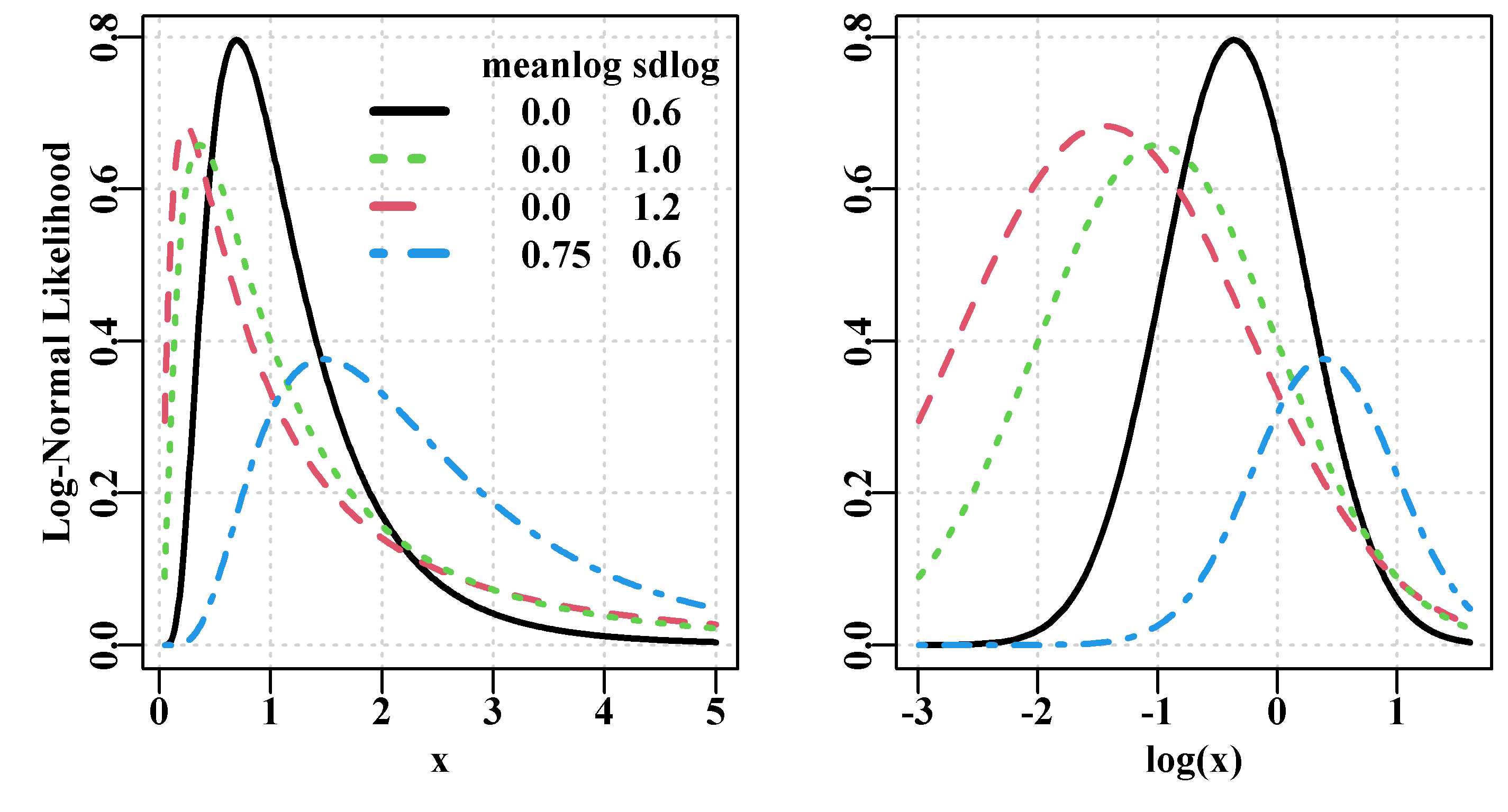
Figure 4.10: Two plots illustrating the Log-Normal probability density function. Left is a group of likelihood distributions for different parameter sets, while right is the log-transformed versions of these first four Log-Normal distributions.
In a similar manner it is possible to generate random numbers from a Log-Normal distribution and, just as before, a log transformation should generate a Normal distribution, as in Figure(4.11)).
set.seed(12354) # plot random log-normal numbers as Fig 4.11
meanL <- 0.7;   sdL <- 0.5  # generate 5000 random log-normal
x <- rlnorm(5000,meanlog = meanL,sdlog = sdL) # values
parset(plots=c(1,2)) # simplifies the plots par() definition
hist(x[x < 8.0],breaks=seq(0,8,0.25),col=0,main="")
meanx <- mean(log(x)); sdx <- sd(log(x))
outstat <- c(exp(meanx-(sdx^2)),exp(meanx),exp(meanx+(sdx^2)/2))
abline(v=outstat,col=c(4,1,2),lwd=3,lty=c(1,2,3))
legend("topright",c("mode","median","bias-correct"),
       col=c(4,1,2),lwd=3,bty="n",cex=1.2,lty=c(1,2,3))
outh <- hist(log(x),breaks=30,col=0,main="")   # approxnormal
hans <- addnorm(outh,log(x)) #MQMF function; try  ?addnorm
lines(hans$x,hans$y,lwd=3,col=1) # type addnorm into the console 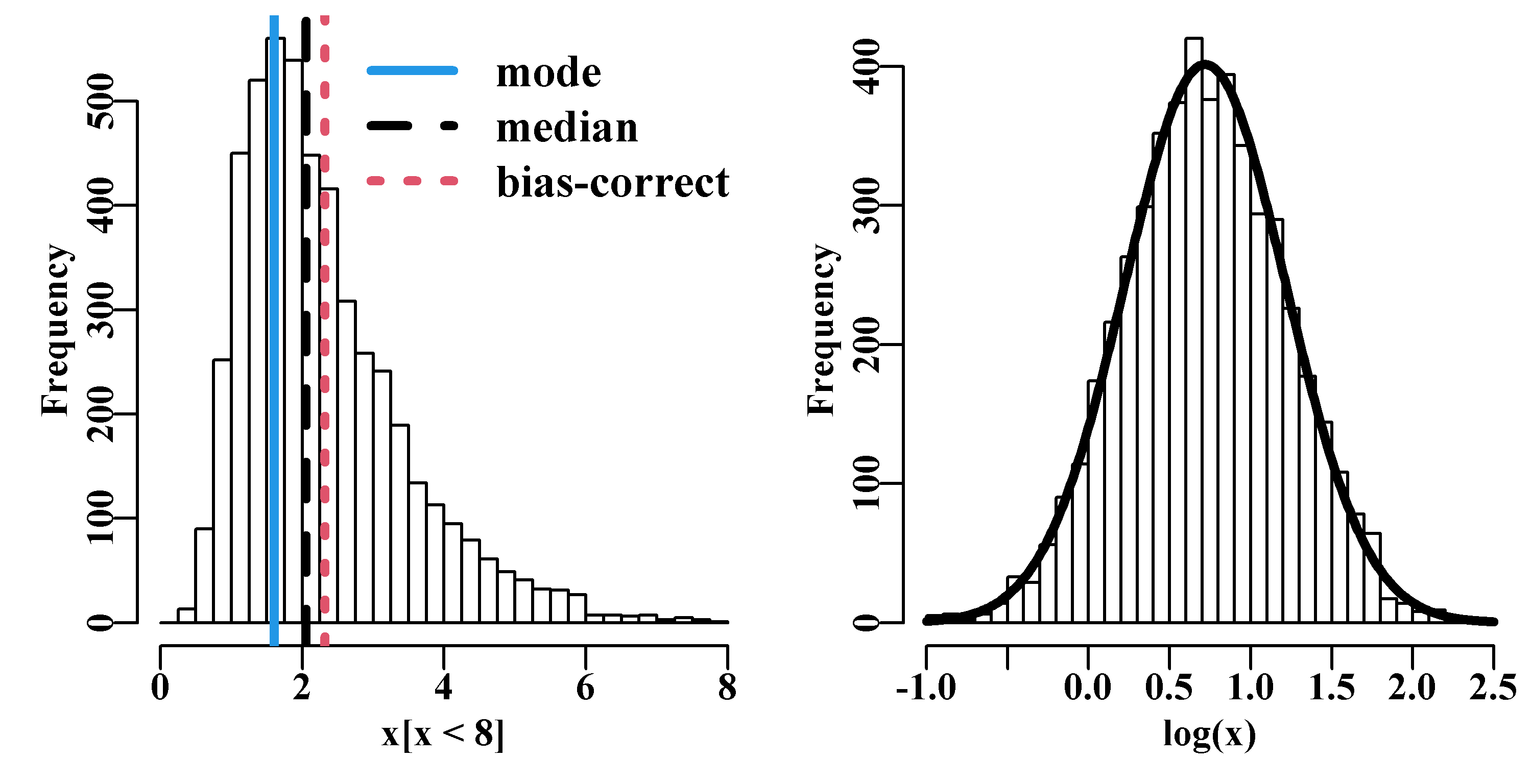
Figure 4.11: A Log-Normal distribution of 5000 random points with meanlog=0.7 and sdlog=0.5 showing the bias-corrected mean, the mode, and the median. On the right is the log-transformed version with a fitted normal distribution.
We can examine the expected statistics from the input parameters, and these can be compared with the parameter estimates made in the variable outstat.
 #examine log-normal propoerties. It is a bad idea to reuse
set.seed(12345) #'random' seeds, use getseed() for suggestions
meanL <- 0.7;   sdL <- 0.5  #5000 random log-normal values then
x <- rlnorm(5000,meanlog = meanL,sdlog = sdL) #try with only 500
meanx <- mean(log(x)); sdx <- sd(log(x))
cat("               Original  Sample \n")
cat("Mode(x)     = ",exp(meanL - sdL^2),outstat[1],"\n")
cat("Median(x)   = ",exp(meanL),outstat[2],"\n")
cat("Mean(x)     = ",exp(meanL + (sdL^2)/2),outstat[3],"\n")
cat("Mean(log(x) =  0.7     ",meanx,"\n")
cat("sd(log(x)   =  0.5     ",sdx,"\n")
# Original Sample
# Mode(x) = 1.568312 1.603512
# Median(x) = 2.013753 2.052606
# Mean(x) = 2.281881 2.322321
# Mean(log(x) = 0.7 0.7001096
# sd(log(x) = 0.5 0.4944283The difference between the median and the mean, the \(+(\sigma^2/2)\) term, is known as the bias-correction term and is attempting to account for the right-ward skew of the distribution by moving the measure of central tendency further to the right away from the mode. The mode appears to sit on the left side of the highest bar, but that merely reflects how R plots histograms (you could add half the bin width to fix this visual problem).
4.7.3 Fitting a Curve using Log-Normal Likelihoods
We can use the spawning stock biomass and subsequent recruitment data from Penn and Caputi (1986), relating to the Australian Exmouth Gulf tiger prawns (Penaeus semisulcatus; MQMF data-set tigers). Stock recruitment relationships often assume Log-Normal residuals (sometimes a Gamma distribution, see later) and normally they would be derived inside a stock assessment model. Penn and Caputi (1986) used a Ricker curve but as an alternative we will attempt to fit a Beverton-Holt stock recruitment curve to these observations (we will examine stock recruitment relationships in more detail in the Static Models chapter). The Beverton-Holt stock recruitment relationship can have more than one form but for this example we will use Equ(4.26):
\[\begin{equation} R_t=\frac{aB_t}{b+B_t}e^{N(0,\sigma^2)} \tag{4.26} \end{equation}\]
where \(R_t\) is the recruitment in year \(t\), \(B_t\) is the spawning stock biomass that gave rise to \(R_t\), \(a\) is the asymptotic maximum recruitment level, and \(b\) is the spawning stock biomass that gives rise to 50% of the maximum recruitment. The residual errors are Log-Normal with \(\mu=0\) and variance \(\sigma^2\), which is estimated when fitting the model to the data. We will continue to use negNLL() but if you examine the code of negNLL() you will see we need to input log-transformed observed recruitment levels and write a short function to calculate the log of predicted recruitment levels. Once again we will use nlm() to minimize the output from negNLL(). When we consider the log-normal residuals (Observed Recruitment / Predicted recruitment) in Table(4.2), notice there are two exceptional residual values, one near 2.04 and the other near 0.44. The potential influence of the low point might bear further investigation as being relatively exceptional events (that appeared in fact, to be influenced by the occurrence of cyclones, Penn and Caputi, 1986).
 # fit a Beverton-Holt recruitment curve to tigers data Table 4.2
data(tigers)   # use the tiger prawn data set
lbh <- function(p,biom) return(log((p[1]*biom)/(p[2] + biom)))
 #note we are returning the log of Beverton-Holt recruitment
pars <- c("a"=25,"b"=4.5,"sigma"=0.4)   # includes a sigma
best <- nlm(negNLL,pars,funk=lbh,observed=log(tigers$Recruit),
            biom=tigers$Spawn,typsize=magnitude(pars))
outfit(best,backtran=FALSE,title="Beverton-Holt Recruitment")
predR <- exp(lbh(best$estimate,tigers$Spawn))
 #note exp(lbh(...)) is the median because no bias adjustment
result <- cbind(tigers,predR,tigers$Recruit/predR)
# nlm solution: Beverton-Holt Recruitment
# minimum : 5.244983
# iterations : 16
# code : 1 gradient close to 0, probably solution
# par gradient
# 1 27.344523 -5.109267e-08
# 2 4.000166 1.270042e-07
# 3 0.351939 1.791807e-06We can plot out the solution to compare the fit with the data visually:
 # Fig 4.12 visual examination of the fit to the tigers data
plot1(tigers$Spawn,predR,xlab="Spawning Biomass","Recruitment",
      maxy=getmax(c(predR,tigers$Recruit)),lwd=2)
points(tigers$Spawn,tigers$Recruit,pch=16,cex=1.1,col=2) 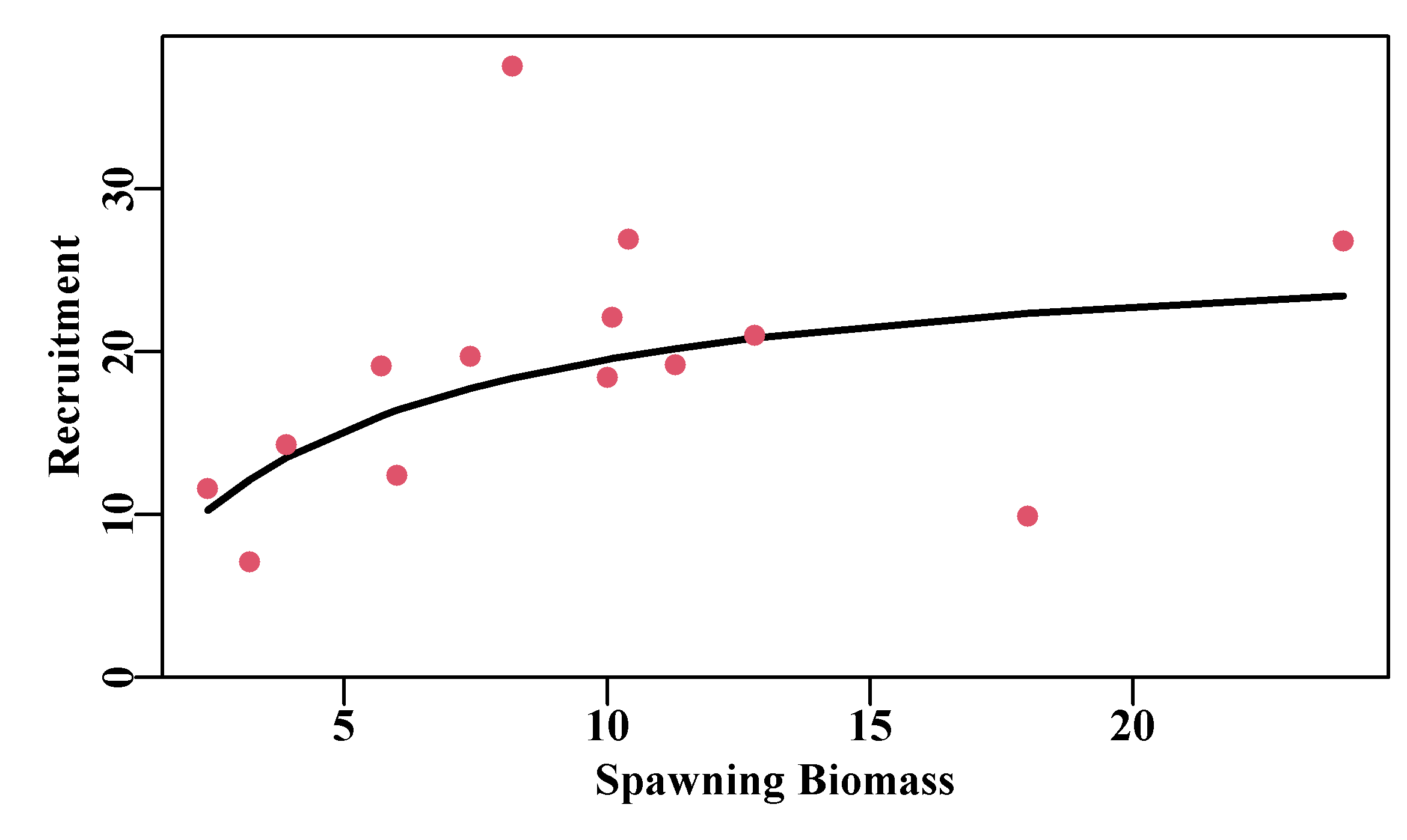
Figure 4.12: The optimum fit to the Exmouth Gulf tiger prawns Beverton-Holt stock recruitment relationship using log-normal likelihoods.
| SpawnB | Recruit | PredR | Residual |
|---|---|---|---|
| 2.4 | 11.6 | 10.254 | 1.1313 |
| 3.2 | 7.1 | 12.153 | 0.5842 |
| 3.9 | 14.3 | 13.499 | 1.0593 |
| 5.7 | 19.1 | 16.068 | 1.1887 |
| 6.0 | 12.4 | 16.406 | 0.7558 |
| 7.4 | 19.7 | 17.750 | 1.1099 |
| 8.2 | 37.5 | 18.379 | 2.0404 |
| 10.0 | 18.4 | 19.532 | 0.9421 |
| 10.1 | 22.1 | 19.587 | 1.1283 |
| 10.4 | 26.9 | 19.749 | 1.3621 |
| 11.3 | 19.2 | 20.195 | 0.9507 |
| 12.8 | 21.0 | 20.834 | 1.0080 |
| 18.0 | 9.9 | 22.373 | 0.4425 |
| 24.0 | 26.8 | 23.438 | 1.1434 |
4.7.4 Fitting a Dynamic Model using Log-Normal Errors
In this example, we will look ahead to an example from the chapter on Surplus Production Models (and previewed in the chapter on Simple Population Models). In particular we will be using what is known as the Schaefer (1954, 1957) surplus production model (Hilborn and Walters, 1992; Polacheck et al, 1993; Prager, 1994; Haddon, 2011). The simplest equations used to describe a Schaefer model involve two terms:
\[\begin{equation} \begin{split} {B_0} &= {B_{init}} \\ {B_{t+1}} &= {B_t}+r{B_t}\left( 1-\frac{{B_t}}{K} \right)-{C_t} \end{split} \tag{4.27} \end{equation}\]
where \(r\) is the intrinsic rate of natural increase (a population growth rate term), \(K\) is the carrying capacity or unfished available biomass, commonly referred to as \(B_0\) (confusingly, here \(B_0\) is simply the initial biomass at \(t = 0\) and \(B_{init}\) could possibly already be depleted below \(K\). \(B_t\) represents the available biomass in year \(t\), with \(B_{init}\) being the biomass in the first year of available data. If the population is unfished then \(B_{init}=K\) but otherwise would constitute a separate model parameter. Finally, \(C_t\) is the total catch taken in year \(t\). Of course, the time-step need not be in years and may need to be some shorter period depending on the biology of the species involved, however, the use of year is common. Notice that there are no error terms in Equ(4.27). This implies that the stock dynamics are deterministic and that the catches are known without error. Estimating the parameters for this model is an example of what is known as using an observation-error estimator.
The simple dynamic model in Equ(4.27) when given the required parameters (\(B_{init}, r,\) and \(K\)), projects the initial biomass forward to generate a time-series of population biomass levels. Such surplus production models can be compared with observations from nature if one has a time-series of relative abundance indices, which may be biomass estimates from surveys or standardized catch-per-unit-effort (CPUE) from fishery dependent data. In the following example we will use the catches and CPUE from a diver caught invertebrate fishery contained in the MQMF data set abdat. The assumption is made that there is a simple linear relationship between the index of relative abundance and the stock biomass:
\[\begin{equation} {I_t}=\frac{C_t}{E_t}=q{B_t}e^{\varepsilon}{ \;\;\;\;\;\; \text{or} \;\;\;\;\;\; } {C_t}=q{E_t}{B_t}e^{\varepsilon} \tag{4.28} \end{equation}\]
where \(I_t\) is the observed CPUE in year \(t\), \(E_t\) is the effort in year \(t\), \(q\) is known as the catchability coefficient (Arreguin-Sanchez, 1996), and \(e^{\varepsilon}\) represents the Log-Normal residual errors on the relationship between the CPUE and the stock biomass. This \(q\) could be estimated directly as a parameter although there is also what is known as a closed form estimate of the same value (Polacheck et al, 1993):
\[\begin{equation} q={e}^{\frac{1}{n}{\sum{log}\left( \frac{{{I}_{t}}}{{{{\hat{B}}}_{t}}} \right)}}=\exp \left( {\frac{1}{n}}\sum{log}\left( \frac{{I}_{t}}{\hat{B}_{t}} \right) \right) \tag{4.29} \end{equation}\]
which is basically the geometric mean of the vector of the observed CPUE divided by the predicted biomass levels in each year. An advantage of using such a closed form is that the model has fewer parameters to estimate when being fitted to data. It also emphasizes that the q parameter is merely a scaling factor that reflects the assumed linear relationship between exploitable biomass and the index of relative abundance. If a non-linear relationship is assumed a more complex representation of the catchability would be required.
The stock recruitment curve fitted in the previous example uses a relatively simple equation and related function as the model to be fitted, but there are no dynamics involved in the modelling. When trying to fit the surplus production model, as described in Equ(4.27) to Equ(4.29), to observed CPUE and catch data, the function that gives rise to the predicted CPUE will need to be more complex as it will need to include the stock dynamics. With simple, non-dynamic models the use of such things as the independent and the dependent variables are relatively straight forward to implement. Here we will illustrate (and reinforce) what is required when fitting a dynamic model to data.
We will use the MQMF data set called abdat, named thus because it contains data on abalone.
data(abdat)  # plot abdat fishery data using a MQMF helper  Fig 4.13
plotspmdat(abdat) # function to quickly plot catch and cpue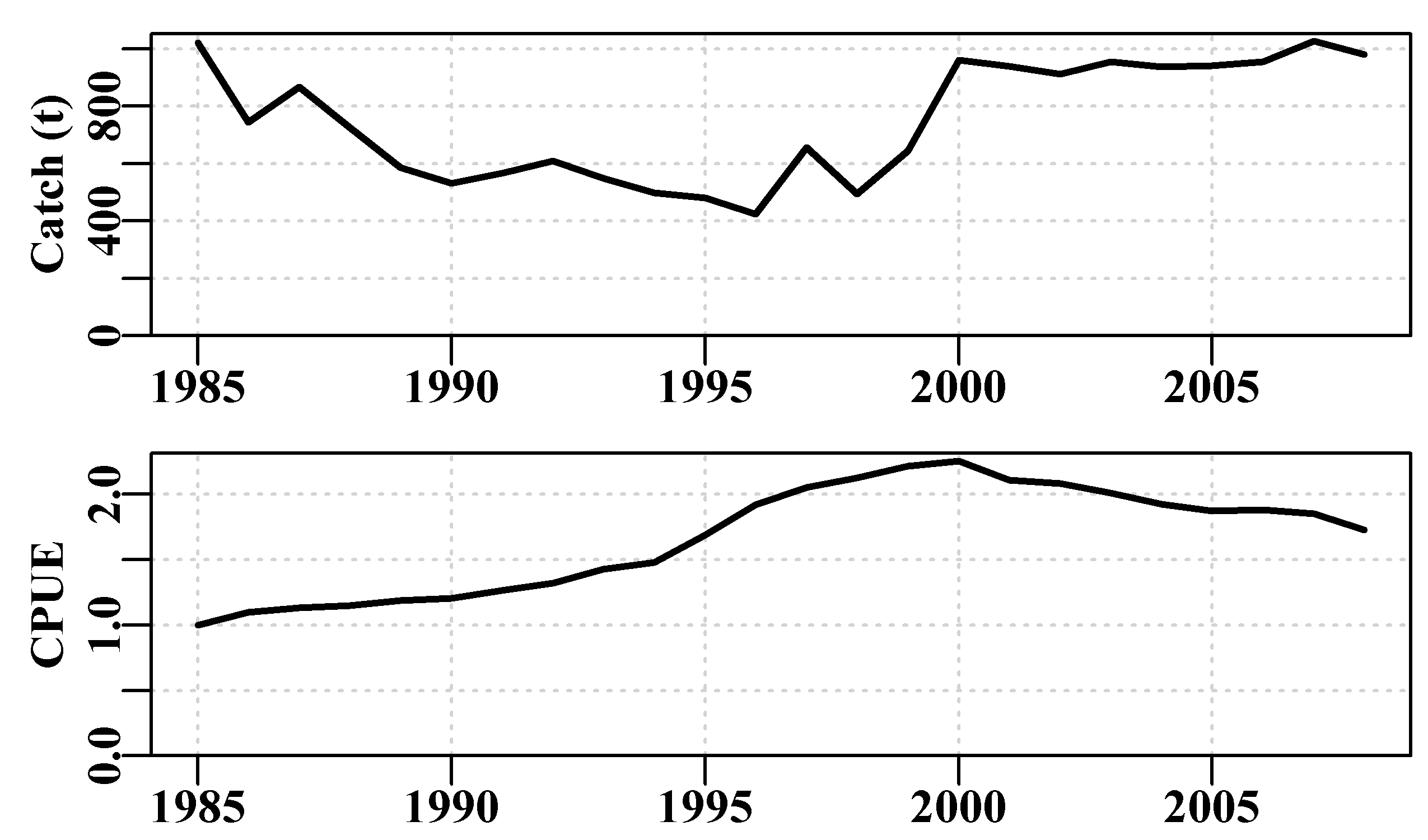
Figure 4.13: The abdat data set plotting the catch and the cpue through time to illustrate their relationship.
We need two functions to use within nlm() to find the optimum parameters. You should examine the code of each and understand how they relate to the equations used. The first is needed to calculate the log of the predicted cpue (we use simpspm()), while the second is used to calculate the -veLL where we are using log-normal residual errors to represent the residuals of the cpue data (so we use negLL(); compare its code with negNLL()). Note the expectation that the model parameters will be log-transformed, we do this as it often leads to greater stability than using the typsize option. You should experiment with this code by trying different starting points. You should carefully examine the code of simpspm and negLL() until you understand how they interact and believe you could repeat this analysis with a different data-set (see the Surplus Production Models chapter).
 # Use log-transformed parameters for increased stability when
 # fitting the surplus production model to the abdat data-set
param <- log(c(r= 0.42,K=9400,Binit=3400,sigma=0.05))
obslog <- log(abdat$cpue) #input log-transformed observed data
bestmod <- nlm(f=negLL,p=param,funk=simpspm,indat=as.matrix(abdat),
               logobs=obslog)  # no typsize, or iterlim needed
 #backtransform estimates, outfit's default, as log-transformed
outfit(bestmod,backtran = TRUE,title="abdat")        # in param
# nlm solution: abdat
# minimum : -41.37511
# iterations : 20
# code : 2 >1 iterates in tolerance, probably solution
# par gradient transpar
# 1 -0.9429555 6.707523e-06 0.38948
# 2 9.1191569 -9.225209e-05 9128.50173
# 3 8.1271026 1.059296e-04 3384.97779
# 4 -3.1429030 -8.161433e-07 0.04316It is always a good idea to plot the observed data against the predicted values from the optimum model. Here we have plotted them on their log-scale to illustrate exactly what was fitted and helps identify which points differed the most from their predicted values. As few have an intuitive grasp of the log-scale it is also a good idea to plot the data and the fit on the nominal scale as well, and, in addition, one would usually plot the residuals to search for patterns.
 # Fig 4.14 Examine fit of predicted to data
predce <- simpspm(bestmod$estimate,abdat) #compare obs vs pred
ymax <- getmax(c(predce,obslog))
plot1(abdat$year,obslog,type="p",maxy=ymax,ylab="Log(CPUE)",
     xlab="Year",cex=0.9)
lines(abdat$year,predce,lwd=2,col=2) 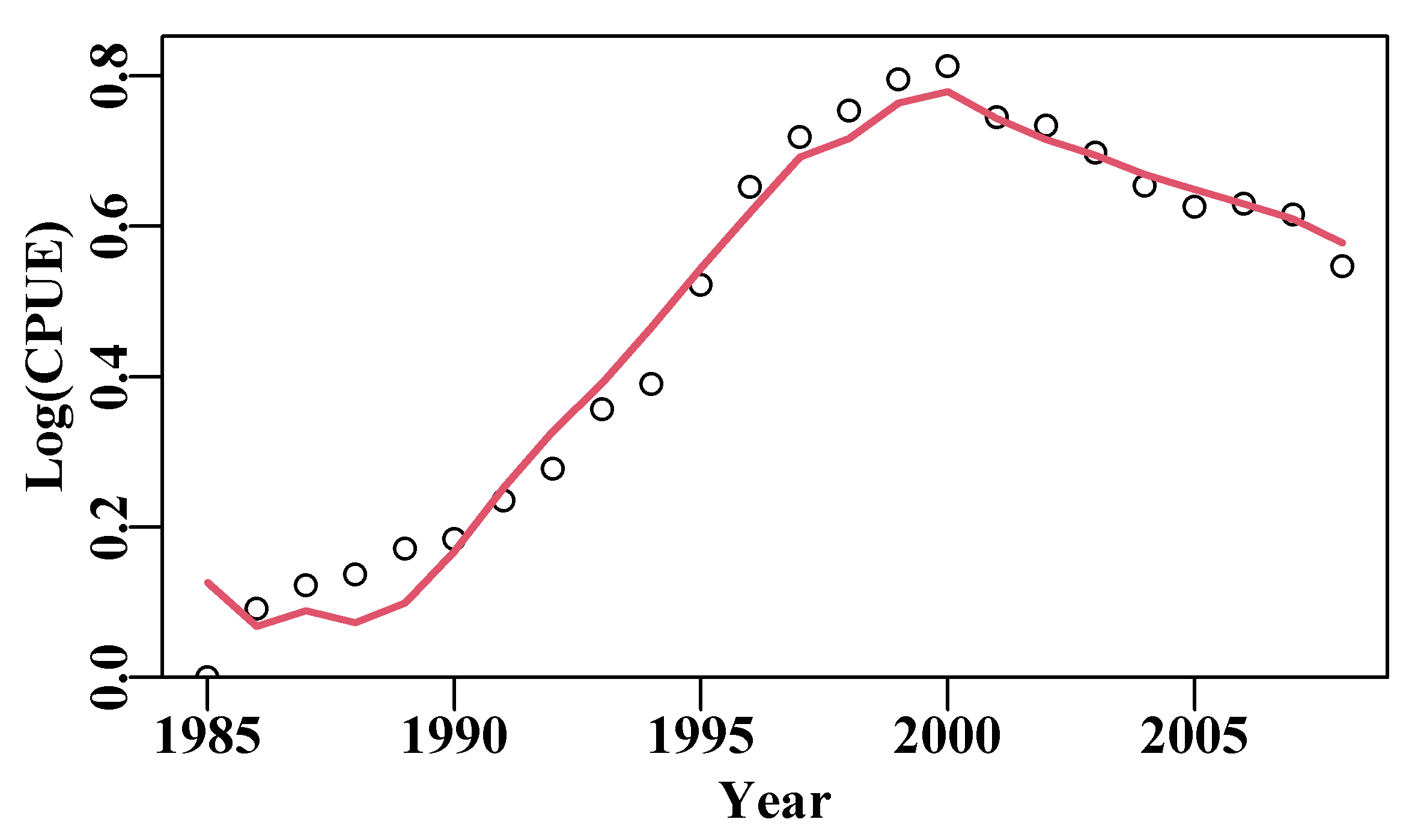
Figure 4.14: The optimum fit of the Schaefer surplus production model to the abdat data set plotted in log-space on the y-axis.
4.8 Likelihoods from the Binomial Distribution
So far, with the Normal and Log-Normal distributions, we have been dealing with likelihoods of particular values of continuous variables (such as spawning biomass and cpue ). But, of course, some observations and events are discrete in nature. Common examples would include an animal being either mature or not, has a tag or not, or similar yes/no situations. In contrast with continuous variables, when likelihoods are calculated for particular values such as the likelihood of seeing m tags in a sample of n observations, using discrete distributions such as the Binomial, they are true probabilities rather than just probability densities. Thus, the complication of understanding likelihoods that are not true probabilities is avoided; which might be why many texts describing maximum likelihood methods tend to start with examples that use the Binomial distribution.
In situations where an observation is true or false (a so-called Bernoulli trial; e.g. a captured fish either has or does not have a tag), and the probability of success out of n observations (trials) is the parameter p, then it would generally be best to use the Binomial distribution to describe observations. The Binomial probability density function generates true probabilities and is characterized by two parameters, n, the number of trials (sample size), and p, the probability of success in a trial (an event/observation proving to be true):
\[\begin{equation} P\left\{ m|n,p \right\}=\left[ \frac{n!}{m!\left( n-m \right)!} \right]{{p}^{m}}{{\left( 1-p \right)}^{\left( n-m \right)}} \tag{4.30} \end{equation}\]
which is read as the probability of \(m\) events proving to be true given \(n\) trials (e.g. \(m\) tags from a sample of \(n\) observations), where \(p\) is the probability of an event being true. The term \((1 - p)\) is often written as \(q\), that is, \((1 – p) = q\). The “!” symbol denotes factorial. The term in the square brackets is the number of combinations that can be formed from \(n\) items taken \(m\) at a time, and is sometimes written as:
\[\begin{equation} \left( \begin{matrix} n \\ m \\ \end{matrix} \right)=\frac{n!}{m!\left( n-m \right)!} \tag{4.31} \end{equation}\]
It is always the case that \(n \geq m\) because one cannot have more successes than trials.
4.8.1 An Example using Binomial Likelihoods
As a first example we might have a population from which a fishery focussed only on males (the Australian Queensland fishery for mud crabs, Scylla serrata, is an example). One might question whether this management strategy negatively affects the sex ratio of legal sized animals from a particular population. In a hypothetical sample of 60 animals if we obtained 40 females and only 20 males would we conclude there had been an impact of the fishery on the sex-ratio? One way to answer such a question would be to examine the relative likelihood of finding such a result (while it is true that Binomial likelihoods are true probabilities we will continue to refer to them also as likelihoods). A typical sex-ratio of 1:1 would mean that we might expect 30 animals to be male from a sample of 60, so, if we declare, for the purposes of this example, that finding a male is a success, we should examine the likelihood of different values of \(m\) (the number of males in our sample of \(n\)) and determine the relative likelihood of finding \(m = 20\) in our sample.
 #Use Binomial distribution to test biased sex-ratio Fig 4.15
n <- 60    # a sample of 60 animals
p <- 0.5   # assume a sex-ration of 1:1
m <- 1:60  # how likely is each of the 60 possibilites?
binom <- dbinom(m,n,p)   # get individual likelihoods
cumbin <- pbinom(m,n,p)  # get cumulative distribution
plot1(m,binom,type="h",xlab="Number of Males",ylab="Probability")
abline(v=which.closest(0.025,cumbin),col=2,lwd=2) # lower 95% CI 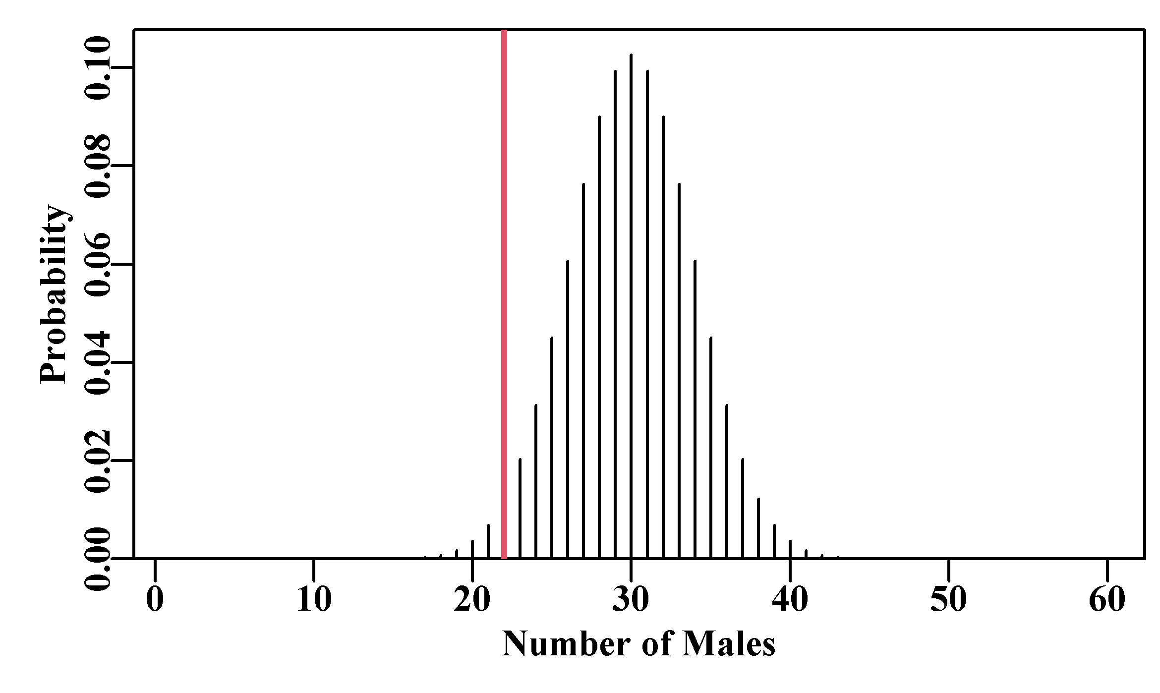
Figure 4.15: A graphical answer to the question of how likely is it to obtain only 20 males in a sample of 60 animals if the sex ratio is 1:1. The vertical red line is the lower bound of the 95% confidence intervals, which suggests that observing only 20 would be unlikely.
One can examine the specific values by examining the contents of binom (individual likelihoods) and cumbin (cumulative Binomial likelihoods). But clearly, if the sex ratio were 1:1 then obtaining fewer than 18 or greater than 42 are both extremely unlikely. Indeed, the chances of getting only 20 males is less that 95%. By examining binom[20] we can see that the likelihood of obtaining exactly 20 males (assuming 1:1 sex ratio) is just over a third of one percent (0.003636) and cumbin[20] tells us that the probability of 20 or less is only 0.006745). We would certainly have grounds for claiming there had been a depression in the sex ratio in the sample from this population. We have also placed a vertical line where the cumulative probability is approximately 0.025. As we are not really interested in the upper limit we could have used 0.05, which would have been more conservative. But such limits have an arbitrary element and what really matters is what is the weight of evidence that the fishing has had no important impact on the sex ratio?
Notice that with relatively large samples the Binomial distribution becomes symmetrical. The tails, however, are shallower than a Normal distribution. For smaller samples, especially with low values of \(p\), the distribution can be highly skewed with a value of zero successes having a specific probability.
Rather than determine whether a given sex ratio is plausible, we could search for the sex ratio (the \(p\) value) that maximized the likelihood of obtaining 20 males out of 60. We would expect it to be 20/60 (0.333…) but there remains interest in knowing the range of plausible values.
 # plot relative likelihood of different p values Fig 4.16
n <- 60  # sample size; should really plot points as each independent
m <- 20  # number of successes = finding a male
p <- seq(0.1,0.6,0.001) #range of probability we find a male
lik <- dbinom(m,n,p)    # R function for binomial likelihoods
plot1(p,lik,type="l",xlab="Prob. of 20 Males",ylab="Prob.")
abline(v=p[which.max(lik)],col=2,lwd=2) # try "p" instead of "l" 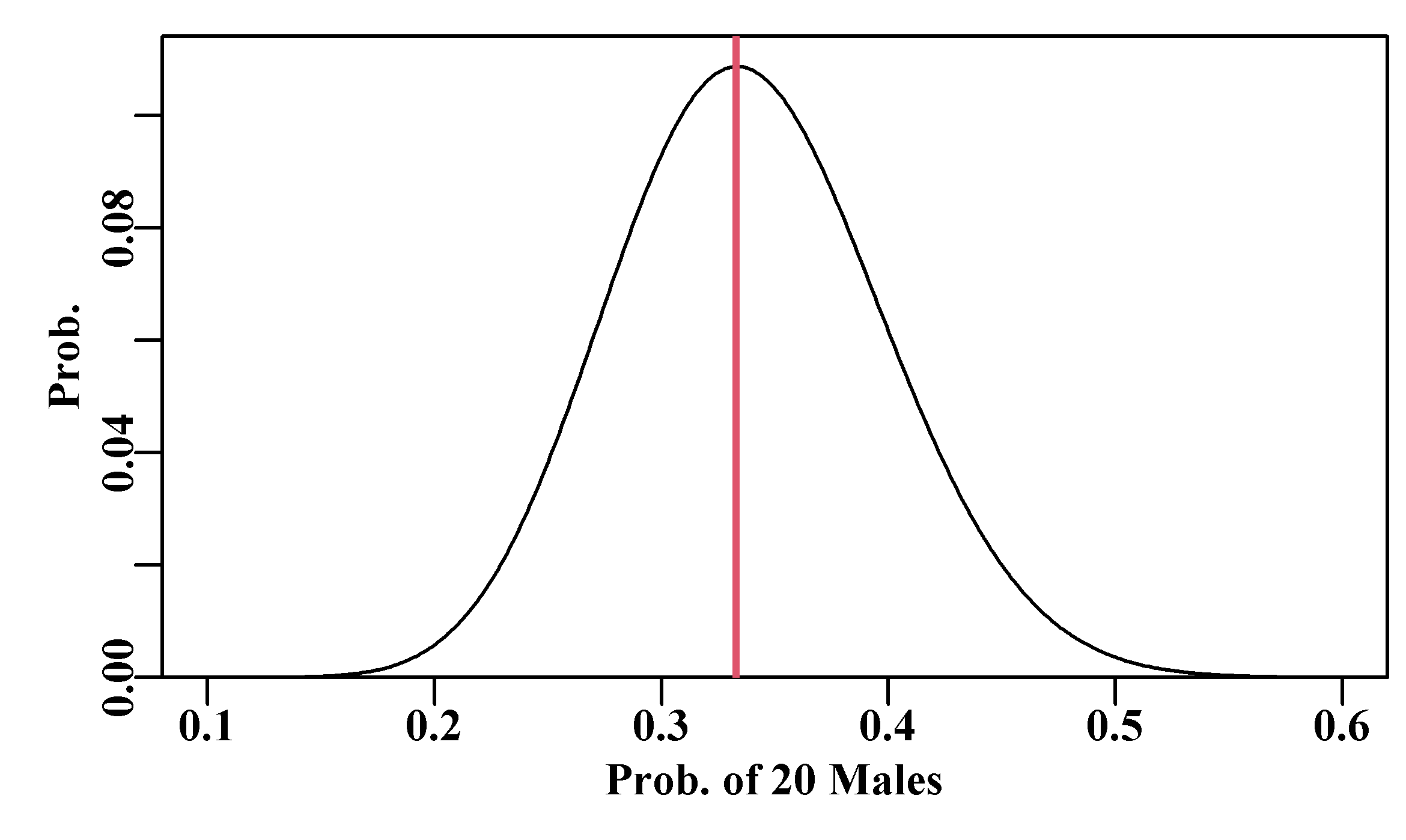
Figure 4.16: Representing the relative likelihood of the proportional sex-ratio when a sample exhibits only 20 males out of 60. Note that the likelihood of there having been a sex-ratio of 0.5 is confirmed as very low.
The use of optimize() (or optimise(), check out ?optimize) is much more efficient than using nlm() when we are only searching for a single parameter. It requires a function whose first term is the value to be minimized or maximized across the interval defined, in this case, by \(p\), hence the simple wrapper function used around dbinom().
 # find best estimate using optimize to finely search an interval
n <- 60; m <- 20  # trials and successes
p <- c(0.1,0.6) #range of probability we find a male
optimize(function(p) {dbinom(m,n,p)},interval=p,maximum=TRUE)
# $maximum
# [1] 0.3333168
#
# $objective
# [1] 0.10872514.8.2 Open Bay Juvenile Fur Seal Population Size
Rather than use a second hypothetical example it is more interesting to use data from a real world case. A suitable study was made on a population of New Zealand fur seal pups (Arctocephalus forsteri) on the Open Bay Islands off the west coast of the South Island of New Zealand (Greaves, 1992; York and Kozlof, 1987). The New Zealand fur seal has been recovering after having been heavily depleted in the nineteenth century, with new haul-out sites now found in both the South and North Island. Exploitation officially ceased in 1894, with complete protection within the New Zealand Exclusive Economic Zone beginning in 1978 (Greaves, 1992). In cooperation with the New Zealand Department of Conservation, Ms Greaves journeyed to and spent a week on one of these offshore islands. She marked 151 fur seal pups by clipping away a small patch of guard hairs on their heads, and then conducted a number of colony walk-throughs to re-sight tagged animals (Greaves, 1992). Each of these walk-throughs constituted a further sample, and differing numbers of animals were found to be tagged in each sample. The question is: What is the size of the fur seal pup population (\(X\)) on the island?
 # Juvenile furseal data-set Greaves, 1992.  Table 4.3
furseal <- c(32,222,1020,704,1337,161.53,31,181,859,593,1125,
             135.72,29,185,936,634,1238,153.99)
columns <- c("tagged(m)","Sample(n)","Population(X)",
             "95%Lower","95%Upper","StErr")
furs <- matrix(furseal,nrow=3,ncol=6,dimnames=list(NULL,columns),
byrow=TRUE) | tagged(m) | Sample(n) | Population(X) | 95%Lower | 95%Upper | StErr |
|---|---|---|---|---|---|
| 32 | 222 | 1020 | 704 | 1337 | 161.53 |
| 31 | 181 | 859 | 593 | 1125 | 135.72 |
| 29 | 185 | 936 | 634 | 1238 | 153.99 |
All the usual assumptions for tagging experiments are assumed to apply; i.e., we are dealing with a closed population—no immigration or emigration, with no natural or tagging mortality over the period of the experiment, no tags are lost, and tagging does not affect the recapture probability of the animals. Finally, the walk-throughs occurred on different days which allowed the pups to move around, so the sightings were all independent of each other. Greaves (1992) estimated all of these effects and accounted for them in her analysis. Having tagged and re-sighted tags, a deterministic answer was found with the Peterson estimator (Caughley, 1977; Seber, 1982):
\[\begin{equation} \frac{{{n}_{1}}}{X}=\frac{m}{n} \;\;\;\;\;\; \therefore \;\;\;\;\;\; \hat{X}=\frac{{{n}_{1}}n}{m} \tag{4.32} \end{equation}\]
where \(n_1\) is the number of tags in the population, \(n\) is the subsequent sample
size, \(m\) is the number of tags recaptured, and \(\hat{X}\) is the estimated population size. An alternative estimator adjusts the counts on the second sample to allow for the fact that in such cases we are dealing with discrete events. This is Bailey’s adjustment (Caughley, 1977):
\[\begin{equation} \hat{X}=\frac{{{n}_{1}}\left( n+1 \right)}{m+1} \tag{4.33} \end{equation}\]
The associated estimate of standard error is used to calculate the approximate 95% confidence intervals using a normal approximation, which leads to symmetrical confidence intervals when using the deterministic equations.
\[\begin{equation} StErr=\sqrt{\frac{n_{1}^{2}\left( n+1 \right)\left( n-m \right)}{{{\left( m+1 \right)}^{2}}\left( m+2 \right)}} \tag{4.34} \end{equation}\]
These equations can be used to confirm the estimates in Table(4.3). However, instead of using the deterministic equations, a good alternative would be to use maximum likelihood to estimate the population size \(\hat{X}\), using the Binomial probability density function.
We are only estimating a single parameter, \(\hat{X}\), the population size, and this entails searching for the population size that maximizes the likelihood of the data. With the Binomial distribution, \(P\left\{ m|n,p \right\}\), Equ(4.30) provides the probability of observing \(m\) tagged individuals from a sample of \(n\) from a population with proportion \(p\) tagged (Snedecor and Cochran, 1967, 1989; Forbes et al, 2011). The proportion of fur seal pups that are marked relates to the population size \(\hat{X}\) and the number of pups originally tagged, which was 151. Hence \(p = 151/\hat{X}\). We will re-analyse the first two samples from Table(4.3).
 # analyse two pup counts 32 from 222, and 31 from 181, rows 1-2 in
 # Table 4.3.   Now set-up storage for solutions
optsol <- matrix(0,nrow=2,ncol=2,
                 dimnames=list(furs[1:2,2],c("p","Likelihood")))
X <- seq(525,1850,1) # range of potential population sizes
p <- 151/X  #range of proportion tagged; 151 originally tagged
m <- furs[1,1] + 1 #tags observed, with Bailey's adjustment
n <- furs[1,2] + 1 # sample size with Bailey's adjustment
lik1 <- dbinom(m,n,p) # individaul likelihoods
 #find best estimate with optimize to finely search an interval
 #use unlist to convert the output list into a vector
 #Note use of Bailey's adjustment (m+1), (n+1) Caughley, (1977)
optsol[1,] <- unlist(optimize(function(p) {dbinom(m,n,p)},p,
                              maximum=TRUE))
m <- furs[2,1]+1;  n <- furs[2,2]+1 #repeat for sample2
lik2 <- dbinom(m,n,p)
totlik <- lik1 * lik2 #Joint likelihood of 2 vectors
optsol[2,] <- unlist(optimize(function(p) {dbinom(m,n,p)},p,
                              maximum=TRUE))
We could certainly tabulate the results but it is clearer to plot them as the likelihood (in this case probability) of each hypothesized population size. Then we can use the \(p\) column within the variable optsol to calculate the optimum population size in each case. The advantage of the plot is that one can immediately see the overlap of the likelihood curves for each sample, and gain an impression that any percentile confidence intervals would not be symmetric.
 # Compare outcome for 2 independent seal estimates Fig 4.17
 # Should plot points not a line as each are independent
plot1(X,lik1,type="l",xlab="Total Pup Numbers",
      ylab="Probability",maxy=0.085,lwd=2)
abline(v=X[which.max(lik1)],col=1,lwd=1)
lines(X,lik2,lwd=2,col=2,lty=3)  # add line to plot
abline(v=X[which.max(lik2)],col=2,lwd=1) # add optimum
 #given p = 151/X, then X = 151/p and p = optimum proportion
legend("topright",legend=round((151/optsol[,"p"])),col=c(1,2),lwd=3,
bty="n",cex=1.1,lty=c(1,3)) 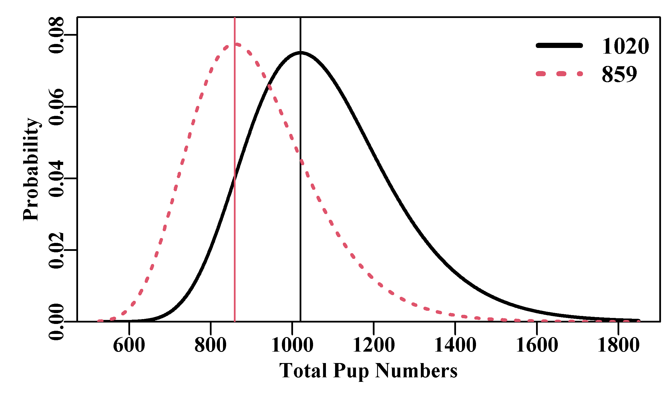
Figure 4.17: The population size versus likelihood distribution for two estimates of fur seal pup population size obtained using tagging experiments where 151 pups were tagged (Greaves, 1992). The right-hand black line is from a single count of 32 tags from 222 pups observed, while the left-hand dashed curve is from a count of 31 tags from 181 observed. The modes (optimum population estimates) are indicated by the vertical lines and in the legend.
4.8.3 Using Multiple Independent Samples
When one has multiple surveys, observations, or samples, or different types of data, and these are independent of one another, it is possible to combine the estimates to improve the overall estimate. Just as with probabilities, the likelihood of a set of independent observations is the product of the likelihoods of the particular observations. Thus, we can multiply the likelihoods from each population size for the two samples we have just examined to obtain a joint likelihood, which in the previous example was put into the variable totlik, Figure(4.18).
 #Combined likelihood from 2 independent samples Fig 4.18
totlik <- totlik/sum(totlik) # rescale so the total sums to one
cumlik <- cumsum(totlik) #approx cumulative likelihood for CI
plot1(X,totlik,type="l",lwd=2,xlab="Total Pup Numbers",
      ylab="Posterior Joint Probability")
percs <- c(X[which.closest(0.025,cumlik)],X[which.max(totlik)],
           X[which.closest(0.975,cumlik)])
abline(v=percs,lwd=c(1,2,1),col=c(2,1,2))
legend("topright",legend=percs,lwd=c(2,4,2),bty="n",col=c(2,1,2),
       cex=1.2)  # now compare with averaged count
m <- furs[3,1];  n <- furs[3,2] # likelihoods for the
lik3 <- dbinom(m,n,p)            # average of six samples
lik4 <- lik3/sum(lik3)  # rescale for comparison with totlik
lines(X,lik4,lwd=2,col=3,lty=2) #add 6 sample average to plot 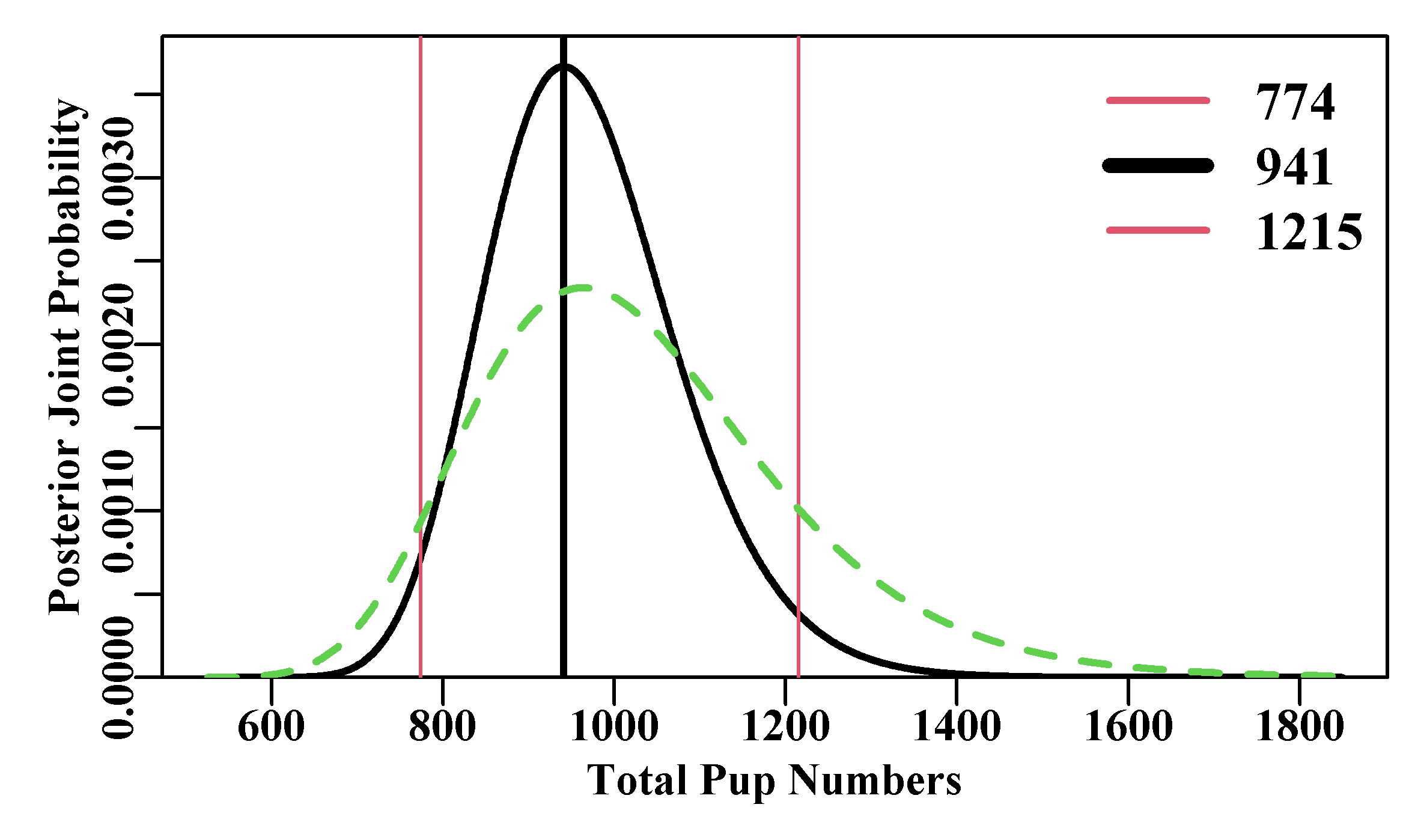
Figure 4.18: The combined likelihood from the first two fur seal pup samples (black line). These have tighter percentile confidence intervals (vertical thin red lines) than the individual samples. The average count and sample size of six samples (green dashed line) remains similar in mean location to the single samples but would have much wider CI. The legend shows the optimum and the 95% percentile CI foir the combined likelihoods curve.
Notice that while the central tendency remains very similar, the 95% confidence intervals from the combination of likelihoods (thin red lines) is tighter and asymmetric around the mean than would be the case from the six combined samples. As with all analyses, as long as the procedures used are defensible, then the analyses can proceed (i.e., in this case it could be argued that the samples were independent, meaning they were taken sufficiently far apart in time that there was no learning the locations of tagged pups, and the pups could move, etc.). There are similarities here to the Bayesian approach of updating a prior probability using likelihoods from new data. Details of actual Bayesian approaches will be given later. The averaging of six samples to obtain average count and sample sizes provides a very similar population estimate but that remains associated with a wider range of uncertainty. Taking averages of such samples is not the optimum analytical strategy.
4.8.4 Analytical Approaches
Some biological processes, such as whether an animal is mature or not, of selected by fishing gear or not, are ideally suited to being analyzed using the Binomial distribution as the underlying basis to observations. However, such processes operate in a cumulative manner so that, for example, with maturity, the percent of a cohort within a population that become mature through time should eventually achieve 100%. Such processes can often be well described using the well known logistic curve. While one could use numerical methods to estimate logistic model parameters it is also possible to use Generalized Linear Models with the Binomial distribution. We will describe these methods in the Static Models chapter that follows this chapter.
4.9 Other Distributions
In the base stats R package (use sessionInfo() to determine the seven base packages loaded) there are probability density functions available for numerous distributions. In fact by typing ?Distributions into the console (with no brackets) you can obtain a list of those available immediately within R. In addition, there is a task view within the CRAN system on distributions that can be found at: https://CRAN.R-project.org/view=Distributions. That task view provides a detailed discussion but also points to a large array of independent packages that provide access to an even wider array of statistical distributions.
Within fisheries science a few of these other distributions are of immediate use. All have probability density functions used when calculating likelihoods (beginning with d, as in dmultinom()) and usually they all have random number generators (beginning with r, as in rgamma()). If you look at the help for a few you should get the idea and see the generalities. Here we will go through some of the details of a few of the more useful for fisheries and ecological work (see also Forbes et al, 2011).
4.10 Likelihoods from the Multinomial Distribution
As seen just above, we use the Binomial distribution when we have situations where there can be two possible outcomes to an observation (true/false, tagged/untagged, mature/immature). However, there are many situations where there are going to be more than two possible discrete outcomes to any observation, and in these situations, we can use the multinomial distribution. Such circumstances can arise when dealing with the frequency distribution within a sample of lengths or ages; e.g. given a random fish its age could lie in just one of a potentially large number of age-classes. In this multivariate sense, the multinomial distribution is an extension of the Binomial distribution. The multinomial is another discrete distribution that provides distinct probabilities and not just likelihoods.
With the Binomial distribution we used \(P(m|n,p)\) to denote the likelihoods. With the multinomial, this needs to be extended so that instead of just two outcomes (one probability \(p\)), we have a probability for each of \(k\) possible outcomes (\(p_k\)) in our sample of \(n\) observations. The probability density function for the multinomial distribution is (Forbes et al, 2011):
\[\begin{equation} P\left\{ {{x}_{i}}|n,{{p}_{1}},{{p}_{2}},...,{{p}_{k}} \right\}=n!\prod\limits_{i=1}^{k}{\frac{\hat{p}_{i}^{{{x}_{i}}}}{x!}} \tag{4.35} \end{equation}\]
where \(x_i\) is the number of times an event of type \(i\) occurs in \(n\) samples (often referred to as trials in the statistical literature), and the \(p_i\) are the separate probabilities for each of the \(k\) types of events possible. The expectation of each type of event is \(E(x_i) = np_i\), where \(n\) is the sample size and \(p_i\) the probability of event type \(i\). Because of the presence of factorial terms in the PDF, which may lead to numerical overflow problems, a log-transformed version of the equation tends to be used:
\[\begin{equation} LL\left\{ {{x}_{i}}|n,{{p}_{1}},...,{{p}_{k}} \right\}=\sum\limits_{j=1}^{n}{log\left( j \right)}+\sum\limits_{i=1}^{k}{\left[ {{x}_{i}}log\left( {{{\hat{p}}}_{i}} \right)-\sum\limits_{j=1}^{x}{log\left( j \right)} \right]} \tag{4.36} \end{equation}\]
In practice, the log-transformed factorial terms \(n!\) and \(x!\), involving the sum of \(log(j)\), where \(j\) steps from 1 to \(n\), and 1 to \(x\), will always be constant and are usually omitted from calculations, in addition the negative log-likelihood is used within minimizers:
\[\begin{equation} -LL\left\{{x_i}|n,{p_1},{p_2},...,{p_k} \right\} \;\;= \;\; -\sum\limits_{i=1}^{k}{\left[ {x_i}log\left( {{\hat{p}}_{i}} \right)\right]} \tag{4.37} \end{equation}\]
There are good reasons why we bother examining simplifications to the probability density functions when there are invariably very serviceable functions for their calculation already developed within R. It is always a good idea to understand what any function we use is doing and that follows from the fact that it is sensible to be aware of the properties of any statistical functions that we want to use in our analyses. In some cases, such as R’s dmultinom() for the multinomial distribution, it’s help page tells us it is not currently vectorized and hence is a little clumsy in its use within fisheries. Instead we will use an R implementation of Equ(4.37) within the MQMF function mnnegLL(). In addition, while the difference in calculation speed is not that important when only dealing with a few hundred observations if one is repeating the calculation of the total log-likelihood for a set of data some millions of times, which is quite possible when using Markov-Chain-Monte-Carlo, or MCMC (sometimes McMC), on fisheries models (see the On Uncertainty chapter), then any way of saving time can be valuable. We will discuss such issues when we address Bayesian and other methods for characterizing uncertainty inherent in our models and data.
4.10.1 Using the Multinomial Distribution
When fitting a model to age- or size-composition data it is common to use the Multinomial distribution to represent the expected distribution of observations among possible categories. We will use an example from a modal analysis study of the growth of juvenile blacklip abalone (Haliotis rubra) from Hope Island in the Derwent Estuary, Tasmania (Helidoniotis and Haddon, 2012). In the sample collected in November 1992, two modes are clear when plotted in 2mm bins.
 #plot counts x shell-length of 2 cohorts   Figure 4.19
cw <- 2  # 2 mm size classes, of which mids are the centers
mids <- seq(8,54,cw) #each size class = 2 mm as in 7-9, 9-11, ...
obs <- c(0,0,6,12,35,40,29,23,13,7,10,14,11,16,11,11,9,8,5,2,0,0,0,0)
 # data from (Helidoniotis and Haddon, 2012)
dat <- as.matrix(cbind(mids,obs)) #xy matrix needed by inthist
parset()  #set up par declaration then use an MQMF function
inthist(dat,col=2,border=3,width=1.8, #histogram of integers
xlabel="Shell Length mm",ylabel="Frequency",xmin=7,xmax=55) 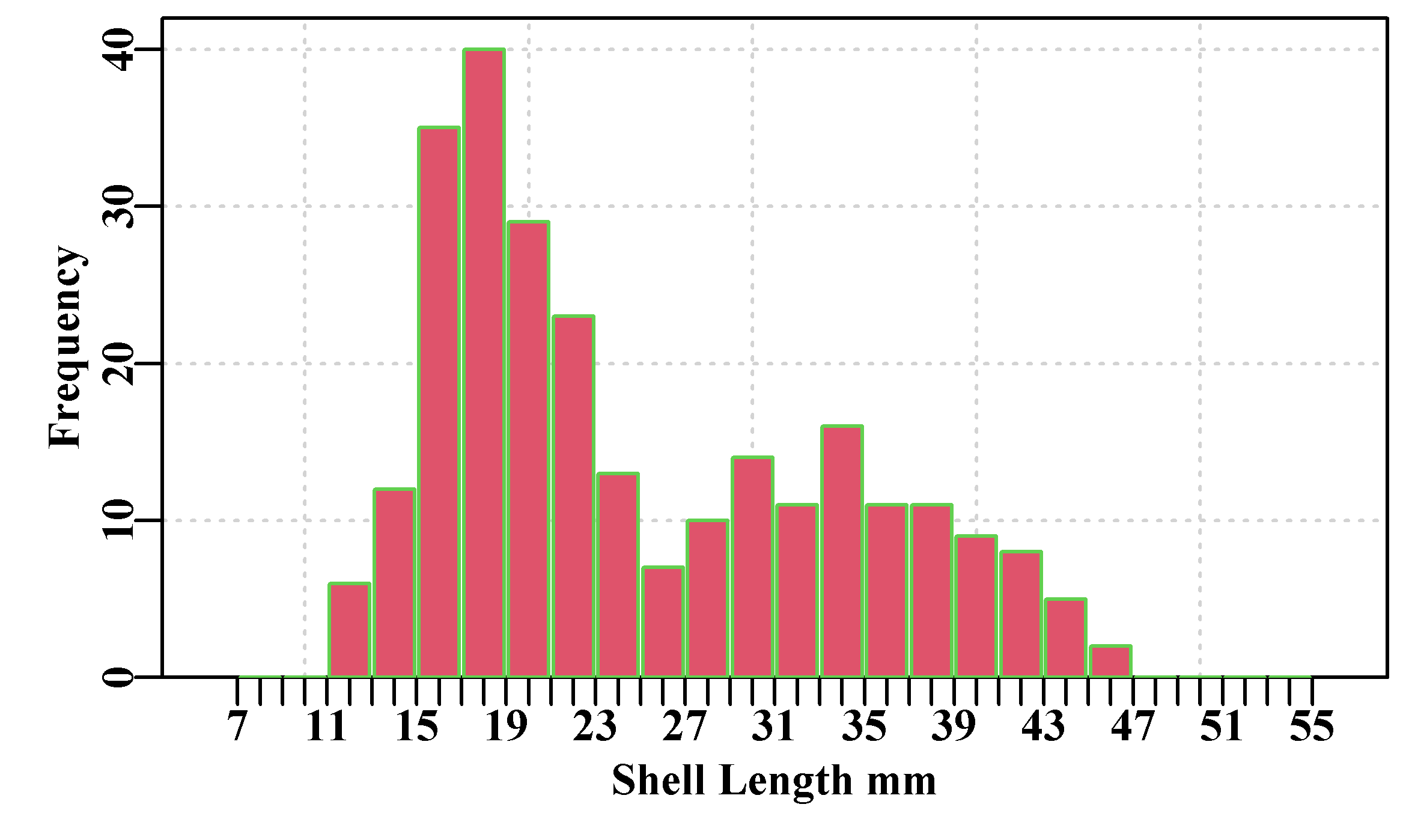
Figure 4.19: The length-frequency counts of a sample of juvenile abalone from the south-east of Tasmania illustrating two modes taken in 1992.
It is assumed that the observable modes in the data relate to distinct cohorts or settlements and we want to estimate the properties of each cohort. A Normal probability density function was used to describe the expected relative frequency of each of the size classes within each mode/cohort, and these are combined to generate the expected relative frequency in each of the \(k\) 2 mm size classes found in the sample (Helidoniotis and Haddon, 2012). There are five parameters required, the mean and standard deviation for each cohort and the proportion of the total number of observations contained in the first cohort (the proportion for the second is obtained through subtraction from 1.0). Thus, using \(\theta = (\mu_c,\sigma_c,\varphi)\), where, in this case there are \(c = 2\) cohorts, we can obtain the expected proportion of observations within each size class. One way would be to calculate the relative likelihood of the center of each 2mm size class and multiply that by the total number in the sample as moderated by the proportion allocated to each cohort, Equ(4.38).
\[\begin{equation} \begin{split} {{{\hat{N}}}_{i}} &= {{\varphi }_{1}}n\sum\limits_{{{S}_{i}}=6}^{56}{\frac{1}{{{\sigma }_{1}}\sqrt{2\pi }}}\exp \left( \frac{-\left( {{S}_{i}}-{{\mu }_{1}} \right)}{2{{\sigma }_{1}}} \right) \\ &+ \left( 1-{{\varphi }_{2}} \right)n\sum\limits_{{{S}_{i}}=6}^{56}{\frac{1}{{{\sigma }_{2}}\sqrt{2\pi }}}\exp \left( \frac{-\left( {{S}_{i}}-{{\mu }_{2}} \right)}{2{{\sigma }_{2}}} \right) \\ {{p}_{i}} &= {{{\hat{N}}}_{i}}/\sum{{{{\hat{N}}}_{i}}} \\ \end{split} \tag{4.38} \end{equation}\]
where \(\hat{N}_i\) is the expected number of observations in each size class \(i\), and \(i\) indexes the number of size classes (here from 7 - 55 mm in steps of 2mm, centered on 8, …, 54). The \(\varphi\) (phi) is the proportion of the total number \(n\) of observations found in cohort 1, the \(\mu_c\) are the mean size of each cohort \(c\), and \(\sigma_c\) refers to their standard deviations. the \(p_i\) in the final row of Equ(4.38) is the expected proportion of observations in size-class \(i\), where the \(S_i\) are the mid-points of each size-class.
Alternatively, and more precisely, we could subtract the cumulative probability for the bottom of each size class \(i\) from the cumulative probability of the top of each size class. However, generally this makes almost no difference in the analysis so here we will concentrate only on the first approach (you could try implementing the alternative yourself to make the comparison as sometimes it is not a good idea to trust everything that is put into print!).
Whichever approach is used, we will need to define two normal distributions and sum their relative contributions. Alternative cumulative statistical distributions to the expected counts, such as the Log-Normal or Gamma, could be used in place of the normal. If no compelling argument can be identified for using one or the other then ideally one would compare the relative fit to the available data obtained by using alternative distributions.
To obtain expected frequencies for comparison with the observed frequencies, it is necessary to constrain the total expected numbers to approximately the same as the numbers observed. The negative log-likelihoods from the multinomial are:
\[\begin{equation} -LL\left\{ N|{\mu_c},{\sigma_c},{\varphi} \right\}=-\sum\limits_{c=1}^{2}\sum\limits_{i=1}^{k}{{N_i}log\left( {{\hat{p}}_i} \right)}=-\sum\limits_{i=1}^{k}{{N_i}log\left( \frac{{{\hat{N}}_i}}{\sum{{{\hat{N}}_i}}} \right)} \tag{4.39} \end{equation}\]
where \(\mu_c\) and \(\sigma_c\) are the mean and standard deviation of the \(c\) cohorts being hypothesized as generating the observed distribution. There are \(k\) size classes and two cohorts \(c\), and \(N_i\) is the observed frequency of size class \(i\), while \(\hat{p}_i\) is the expected proportion within size class \(i\) from the combined normal distributions. The objective would be to minimize the negative log-likelihood to find the optimum combination of the \(c\) Normal distribution parameters and \(\varphi\).
 #cohort data with 2 guess-timated normal curves Fig 4.20
parset()  # set up the required par declaration
inthist(dat,col=0,border=8,width=1.8,xlabel="Shell Length mm",
        ylabel="Frequency",xmin=7,xmax=55,lwd=2)  # MQMF function
 #Guess normal parameters and plot those curves on histogram
av <- c(18.0,34.5)    # the initial trial and error means and
stdev <- c(2.75,5.75)  # their standard deviations
prop1 <- 0.55       #  proportion of observations in cohort 1
n <- sum(obs) #262 observations, now calculate expected counts
cohort1 <- (n*prop1*cw)*dnorm(mids,av[1],stdev[1]) # for each
cohort2 <- (n*(1-prop1)*cw)*dnorm(mids,av[2],stdev[2])# cohort
 #(n*prop1*cw) scales likelihoods to suit the 2mm class width
lines(mids,cohort1,lwd=2,col=1)
lines(mids,cohort2,lwd=2,col=4) 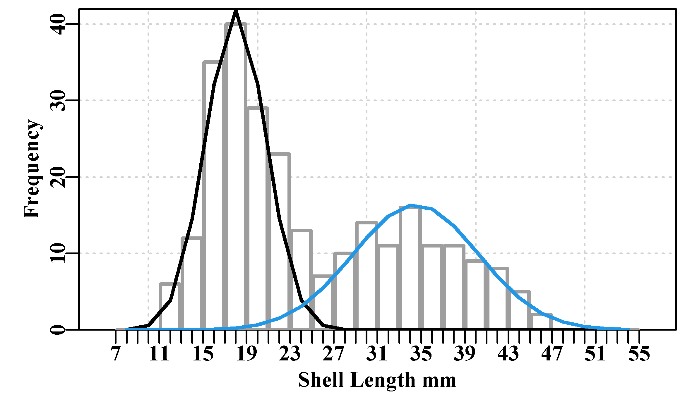
Figure 4.20: Two Normal distributions from initial parameter guesses imposed upon the length-frequency counts of juvenile abalone from southern Tasmania sampled in 1992.
The central estimates for the initial trial and error guesses for the two modes appear reasonable but the spread in the left hand cohort appears too small and the proportional allocation between the cohorts appears biased towards the first cohort. Being based upon proportions, which alter values in non-linear ways the search for an optimal likelihood can be sensitive to the starting values. We can search for a more optimal parameter set by applying nlm() to a wrapper function that is used to generate an estimate of the negative log-likelihood for the multinomial, as defined in Equ(4.39). As previously, we need a function to generate the predicted numbers of observations in each size class, in MQMF we have called it predfreq(). We also need a wrapper function that will calculate the negative log-likelihood using the predfreq() function, here we have called this wrapper() (see code chunk below). In developing the predfreq() function we have required that the parameters be ordered with the means of each cohort being fitted coming first, followed by their standard deviations, and then the proportions allocated to all but the last cohort coming at the end. This allows the algorithm to find the required parameters in their defined places. Thus, for a three cohort problem, in R we would have \(pars={c(\mu_1,\mu_2,\mu_3,\sigma_1,\sigma_2,\sigma_3,\varphi_1,\varphi2)}\). We have also included the option of using the cumulative Normal probability density.
 #wrapper function for calculating the multinomial log-likelihoods
 #using predfreq and mnnegLL, Use ? and examine their code
wrapper <- function(pars,obs,sizecl,midval=TRUE) {
  freqf <- predfreq(pars,sum(obs),sizecl=sizecl,midval=midval)
  return(mnnegLL(obs,freqf))
} # end of wrapper which uses MQMF::predfreq and MQMF::mnnegLL
mids <- seq(8,54,2) # each size class = 2 mm as in 7-9, 9-11, ...
av <- c(18.0,34.5)   # the trial and error means and
stdev <- c(2.95,5.75)  # standard deviations
phi1 <- 0.55      # proportion of observations in cohort 1
pars <-c(av,stdev,phi1)  # combine parameters into a vector
wrapper(pars,obs=obs,sizecl=mids) # calculate total -veLL
# [1] 708.3876 # First use the midpoints
bestmod <- nlm(f=wrapper,p=pars,obs=obs,sizecl=mids,midval=TRUE,
typsize=magnitude(pars))
outfit(bestmod,backtran=FALSE,title="Using Midpts"); cat("\n")
#Now use the size class bounds and cumulative distribution
#more sensitive to starting values, so use best pars from midpoints
X <- seq((mids[1]-cw/2),(tail(mids,1)+cw/2),cw)
bestmodb <- nlm(f=wrapper,p=bestmod$estimate,obs=obs,sizecl=X,
midval=FALSE,typsize=magnitude(pars))
outfit(bestmodb,backtran=FALSE,title="Using size-class bounds") # nlm solution: Using Midpts
# minimum : 706.1841
# iterations : 27
# code : 1 gradient close to 0, probably solution
# par gradient
# 1 18.3300619 6.382071e-06
# 2 33.7907454 4.471337e-06
# 3 3.0390094 -2.835616e-05
# 4 6.0306017 6.975113e-06
# 5 0.5763628 7.515178e-05
#
# nlm solution: Using size-class bounds
# minimum : 706.1815
# iterations : 24
# code : 1 gradient close to 0, probably solution
# par gradient
# 1 18.3299573 2.363054e-06
# 2 33.7903327 -4.690083e-06
# 3 2.9831560 2.217978e-05
# 4 6.0030194 -2.880512e-05
# 5 0.5763426 -5.187824e-05Now plot these optimal solutions against the original data. Plotting the data is simple enough but then we need to pull out the optimal parameters in each case and calculate the implied normal distributions for each.
 #prepare the predicted Normal distribution curves
pars <- bestmod$estimate # best estimate using mid-points
cohort1 <- (n*pars[5]*cw)*dnorm(mids,pars[1],pars[3])
cohort2 <- (n*(1-pars[5])*cw)*dnorm(mids,pars[2],pars[4])
parsb <- bestmodb$estimate # best estimate with bounds
nedge <- length(mids) + 1  # one extra estimate
cump1 <- (n*pars[5])*pnorm(X,pars[1],pars[3])#no need to rescale
cohort1b <- (cump1[2:nedge] - cump1[1:(nedge-1)])
cump2 <- (n*(1-pars[5]))*pnorm(X,pars[2],pars[4])  # cohort 2
cohort2b <- (cump2[2:nedge] - cump2[1:(nedge-1)])
#plot the alternate model fits to cohorts Fig 4.21
parset() # set up required par declaration; then plot curves
pick <- which(mids < 28)
inthist(dat[pick,],col=0,border=8,width=1.8,xmin=5,xmax=28,
xlabel="Shell Length mm",ylabel="Frequency",lwd=3)
lines(mids,cohort1,lwd=3,col=1,lty=2) # have used setpalette("R4")
lines(mids,cohort1b,lwd=2,col=4) # add the bounded results
label <- c("midpoints","bounds") # very minor differences
legend("topleft",legend=label,lwd=3,col=c(1,4),bty="n",
cex=1.2,lty=c(2,1)) 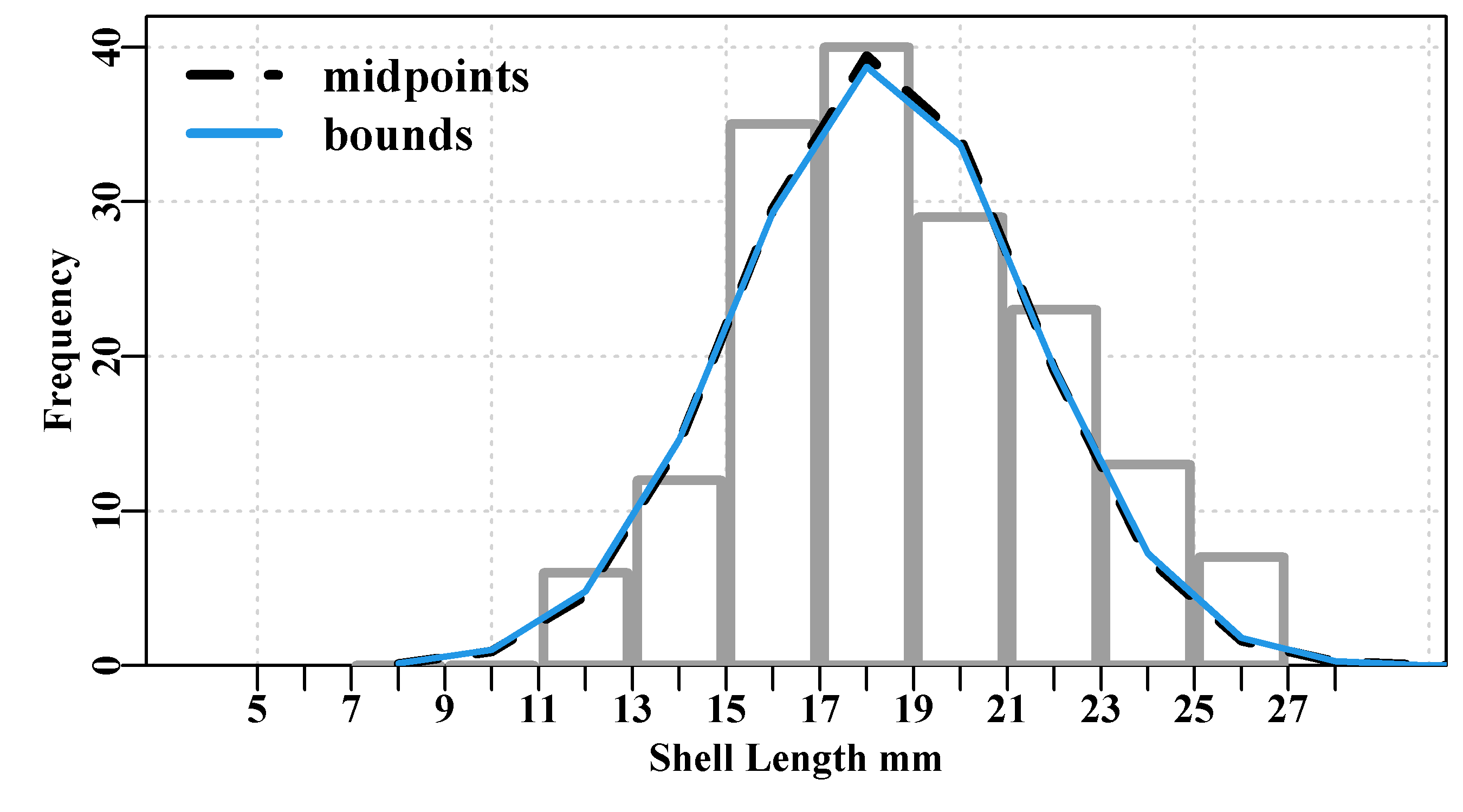
Figure 4.21: The optimum fit to the left-hand mode of the length-frequency information. The differences in parameter values between using size-class midpts or bounds occurs at the fourth decimal place. The difference in the right-hand mode was so small as not to be discernible.
In this case the parameters obtained when using the mid-points of the different size classes barely differ from the parameters obtained when using the upper and lower bounds of each size class with the resulting Normal curves almost completely overlapping. We can see the details of these fits by listing the observed counts and the predicted counts, in each case, and the differences between the predicted and observed numbers in each size class. As in Figure(4.21), the numbers themselves illustrate more clearly the closeness of the two approaches, Table(4.4). The use of the upper and lower bounds is strictly more correct, but in practice it often makes little difference.
A different strategy for fitting modal distributions to mixed distributions can be found in Venebles and Ripley (2002, p436). Their approach is more sophisticated and elegant in that they uses analytical gradients to assist the model fitting process. Hopefully it is clear that for almost any analytical problem there will be more than one way to solve it. Using numerical methods often entails exploring alternative methods in the search for a solution.
 # setup table of results for comparison of fitting strategies
predmid <- rowSums(cbind(cohort1,cohort2))
predbnd <- rowSums(cbind(cohort1b,cohort2b))
result <- as.matrix(cbind(mids,obs,predmid,predbnd,predbnd-predmid))
colnames(result) <- c("mids","Obs","Predmid","Predbnd","Difference")
result <- rbind(result,c(NA,colSums(result,na.rm=TRUE)[2:5])) | mids | Obs | Predmid | Predbnd | Difference |
|---|---|---|---|---|
| 8 | 0 | 0.1244 | 0.1487 | 0.0243 |
| 10 | 0 | 0.9323 | 1.0429 | 0.1106 |
| 12 | 6 | 4.5513 | 4.8236 | 0.2722 |
| 14 | 12 | 14.4344 | 14.6975 | 0.2631 |
| 16 | 35 | 29.7390 | 29.5255 | -0.2135 |
| 18 | 40 | 39.8899 | 39.2110 | -0.6789 |
| 20 | 29 | 35.1656 | 34.7612 | -0.4044 |
| 22 | 23 | 21.2938 | 21.4733 | 0.1795 |
| 24 | 13 | 10.8868 | 11.2236 | 0.3368 |
| 26 | 7 | 8.0156 | 8.1948 | 0.1792 |
| 28 | 10 | 9.5120 | 9.5510 | 0.0390 |
| 30 | 14 | 12.0774 | 12.0505 | -0.0268 |
| 32 | 11 | 14.0533 | 13.9954 | -0.0579 |
| 34 | 16 | 14.6763 | 14.6094 | -0.0669 |
| 36 | 11 | 13.7320 | 13.6777 | -0.0543 |
| 38 | 11 | 11.5103 | 11.4832 | -0.0270 |
| 40 | 9 | 8.6431 | 8.6454 | 0.0023 |
| 42 | 8 | 5.8142 | 5.8368 | 0.0226 |
| 44 | 5 | 3.5038 | 3.5337 | 0.0298 |
| 46 | 2 | 1.8916 | 1.9184 | 0.0268 |
| 48 | 0 | 0.9149 | 0.9339 | 0.0191 |
| 50 | 0 | 0.3964 | 0.4077 | 0.0113 |
| 52 | 0 | 0.1538 | 0.1596 | 0.0058 |
| 54 | 0 | 0.0535 | 0.0560 | 0.0025 |
| 262 | 261.9656 | 261.9607 | -0.0049 |
4.11 Likelihoods from the Gamma Distribution
The Gamma distribution is generally less well known than the statistical distributions we have considered in previous sections. Nevertheless, the gamma distribution is becoming more commonly used in fisheries modelling and in simulation ; practical examples can be found in the context of length-based population modelling (Sullivan et al, 1990; Sullivan, 1992). The probability density function for the Gamma distribution has two parameters, a scale parameter b (\(b < 0\); an alternative sometimes used is \(\lambda\), where \(\lambda < {1/b}\)), and a shape parameter c (\(c > 0\)). The distribution extends over the range of \(0 \leq{x} \leq{\infty}\) (i.e. no negative values). The expectation or mean of the distribution, \(E(x)\), relates the two parameters, the scale \(b\) and the shape \(c\). Thus:
\[\begin{equation} E{( x )}=bc \;\;\;\ \text{or} \;\;\;\ c=\frac{E{( x )}}{b} \tag{4.40} \end{equation}\]
The probability density function for calculating the individual likelihoods for the Gamma distribution is (Forbes et al, 2011):
\[\begin{equation} L\left\{ x \vert b,c \right\}=\frac{{{\left( \frac{x}{b} \right)}^{( c-1 )}}{{e}^{\frac{-x}{b}}}}{b\Gamma (c)} \tag{4.41} \end{equation}\]
where \(x\) is the value of the variate, \(b\) is the scale parameter, \(c\) is the shape parameter, and \(\Gamma(c)\) is the gamma function for the \(c\) parameter. In cases where \(c\) takes on integer values the distribution is also known as the Erlang distribution where the gamma function (\(\Gamma(c)\)) is replaced by factorial \((c-1)!\) (Forbes et al, 2011):
\[\begin{equation} L\left\{ x|b,c \right\}=\frac{{{\left( \frac{x}{b} \right)}^{\left( c-1 \right)}}{{e}^{\frac{-x}{b}}}}{b\left( c-1 \right)!} \tag{4.42} \end{equation}\]
As usual with likelihood calculations, to avoid computational issues of over- and under-flow it is standard to calculate the log-likelihoods, and more specifically negative log-likelihoods. The use of log-likelihoods is invariably more risk-averse:
\[\begin{equation} -LL\{x|b,c\}= -\left[ \left( (c-1)log\left( \frac{x}{b} \right)-\frac{x}{b} \right) -\{log{(b)}+ log{\left( \Gamma \left( c \right) \right)} \} \right] \tag{4.43} \end{equation}\]
For multiple observations this enables their summation rather than product, but it still requires the calculation of the log-gamma function \(log(\Gamma (c))\). Fortunately for us, there is both a gamma() and a lgamma() function defined in R.
The Gamma distribution (not to be confused with the gamma function, \(\Gamma\)) is extremely flexible, ranging in shape from effectively an inverse curve, through a right-hand skewed curve, to approximately normal in shape. Its flexibility makes it a very useful function for simulations, Figure(4.22).
 #Illustrate different Gamma function curves  Figure 4.22
X <- seq(0.0,10,0.1) #now try different shapes and scale values
dg <- dgamma(X,shape=1,scale=1)
plot1(X,dg,xlab = "Quantile","Probability Density")
lines(X,dgamma(X,shape=1.5,scale=1),lwd=2,col=2,lty=2)
lines(X,dgamma(X,shape=2,scale=1),lwd=2,col=3,lty=3)
lines(X,dgamma(X,shape=4,scale=1),lwd=2,col=4,lty=4)
legend("topright",legend=c("Shape 1","Shape 1.5","Shape 2",
       "Shape 4"),lwd=3,col=c(1,2,3,4),bty="n",cex=1.25,lty=1:4)
mtext("Scale c = 1",side=3,outer=FALSE,line=-1.1,cex=1.0,font=7) 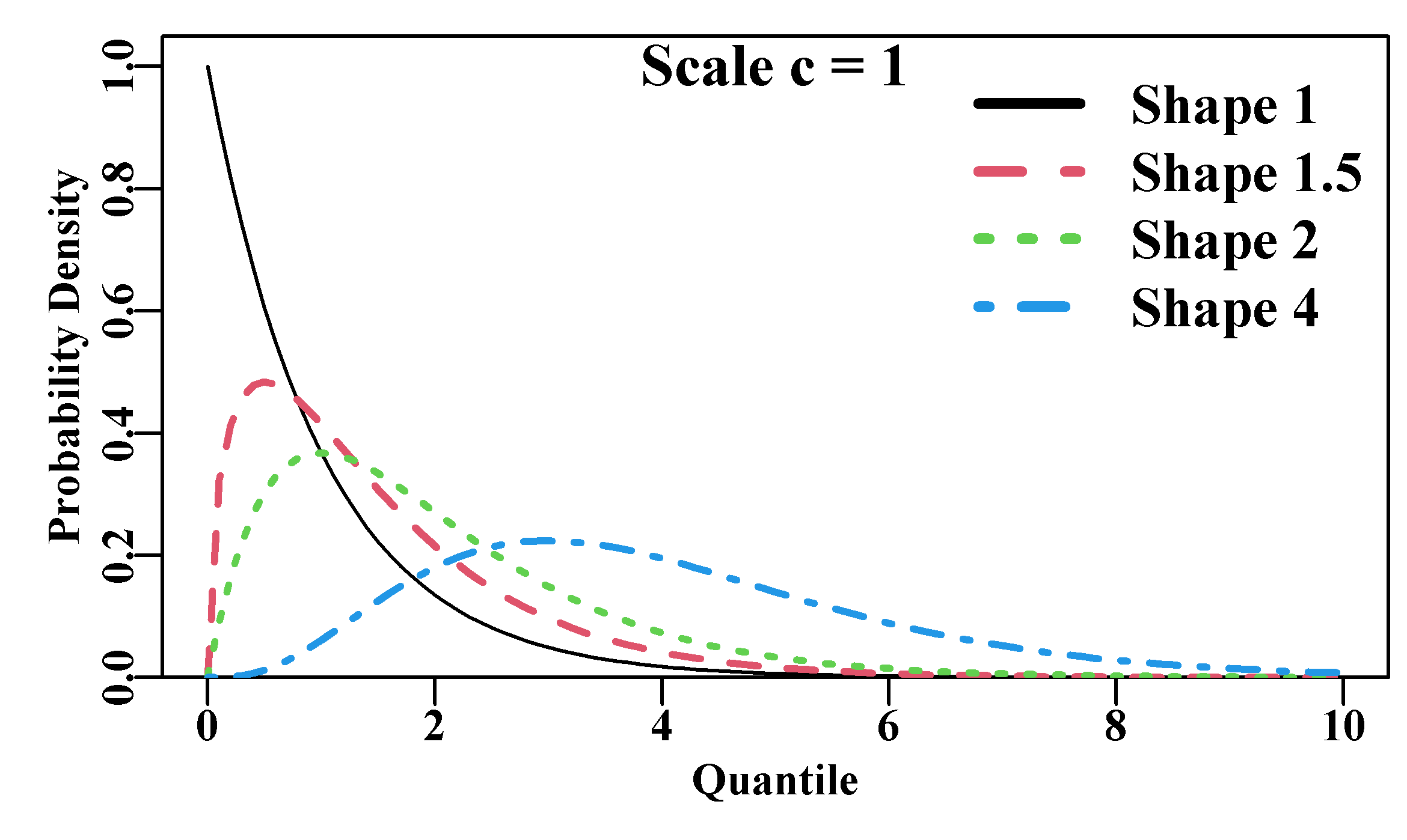
Figure 4.22: Different Gamma distributions all with a scale c = 1.0.
In the section on the Multinomial distribution we used Normal distributions to describe the expected distribution of lengths within a cohort. It is also possible that the growth pattern of a species might be better described using a Gamma distribution.
4.12 Likelihoods from the Beta Distribution
The Beta distribution is only defined for values of a variable between 0.0 and 1.0. This makes it another very useful distribution for use in simulations because it is relatively common that one is required to sample from a distribution of values between 0 to 1, without the possibility of obtaining values beyond those limits, Figure(4.23). It is recommended that you explore the possibilities available within R. In the chapter On Uncertainty we will be using the multi-variate Normal distribution, which requires the use of an extra R package. The array of distributions available for analysis and simulation is very large. Exploration would be the best way of discovering their properties.
 #Illustrate different Beta function curves. Figure 4.23
x <- seq(0, 1, length = 1000)
parset()
plot(x,dbeta(x,shape1=3,shape2=1),type="l",lwd=2,ylim=c(0,4),
     yaxs="i",panel.first=grid(), xlab="Variable 0 - 1",
     ylab="Beta Probability Density - Scale1 = 3")
bval <- c(1.25,2,4,10)
for (i in 1:length(bval))
  lines(x,dbeta(x,shape1=3,shape2=bval[i]),lwd=2,col=(i+1),lty=c(i+1))
legend(0.5,3.95,c(1.0,bval),col=c(1:7),lwd=2,bty="n",lty=1:5) 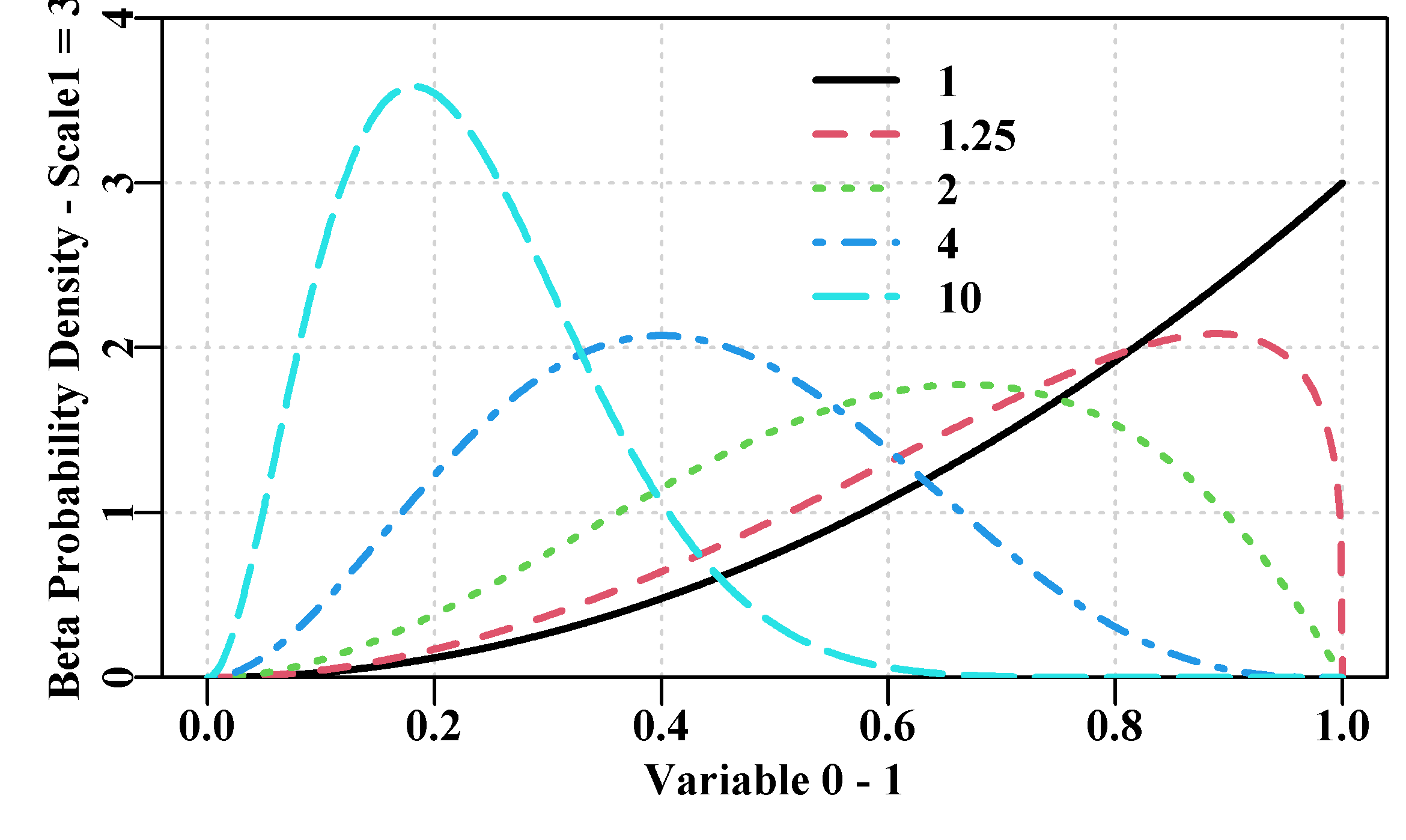
Figure 4.23: Different Beta probability density distributions all with a shape1 value = 3.0, and with values of shape2 ranging from 1 to 10.
4.13 Bayes’ Theorem
4.13.1 Introduction
There has been an expansion in the use of Bayesian statistics in fisheries science (McAllister et al, 1994; McAllister and Ianelli, 1997; Punt and Hilborn, 1997; see Dennis, 1996, for an opposing view; more recently see Winker et al, 2018). An excellent book relating to the use of these methods was produced by Gelman et al (2014). Here we are not going to attempt a review of the methodology as it is used in fisheries; a good introduction can be found in Punt and Hilborn (1997), and there are many more recent examples. Instead, we will concentrate upon the foundation of Bayesian methods as used in fisheries and draw some comparisons with maximum likelihood methods. Details of how one can approach the use of these methods are provided in the chapter On Uncertainty.
Conditional probabilities are used to describe situations where one is interested in the probability that a particular event, say \(B_i\), will occur given that an event \(A\) has already happened. The notation for this expression is \(P(B_i|A)\), where the vertical line, “|”, refers to the notion of given.
Bayes’ theorem is based around a manipulation of such conditional probabilities. Thus, if a set of n events, labelled \(B_i\), occur given that an event \(A\) has occurred, then we can formally develop Bayes’ theorem. First, we consider the probability of observing a particular \(B_i\) given that \(A\) has occurred:
\[\begin{equation} P\left( {{B}_{i}}|A \right)=\frac{P\left( A \& B_i \right)}{P\left( A \right)} \tag{4.44} \end{equation}\]
That is, the probability of \(B_i\) occurring given the \(A\) has occurred is the probability of both \(A\) and \(B_i\) occur divided by the probability that \(A\) occurs. In an equivalent manner we can consider the conditional probability of the event \(A\) given the occurrence of the \(B_i\) event.
\[\begin{equation} P\left( {A}|{B_i} \right)=\frac{P\left( {A} \& {B}_{i} \right)}{P\left( {B}_{i} \right)} \tag{4.45} \end{equation}\]
Those two conditional probabilities can be rearranged to give:
\[\begin{equation} P\left( A|{B_i} \right)P\left( {B}_{i} \right)=P\left( A \& {B}_{i} \right) \tag{4.46} \end{equation}\]
We can use this to replace the \(P(A\&{B_i})\) term in the Equ(4.44) to obtain the classical Bayes’ Theorem:
\[\begin{equation} P\left({B_i}|A\right)=\frac{P\left(A|{B_i}\right)P\left({B_i}\right)}{P\left(A\right)} \tag{4.47} \end{equation}\]
If we translate this seemingly obscure theorem such that \(A\) represents data obtained from nature, and the various \(B_i\) as the separate hypotheses one might use to explain the data (where an hypothesis is a model plus a vector of parameters, \(\theta\)), then we can derive the form of Bayes’ Theorem as it is used in fisheries. Thus, the \(P(A|B_i)\) is just the likelihood of the the data \(A\) given the model plus parameters \(B_i\) (the hypothesis); we are already familiar with this from maximum likelihood theory and practice. A new bit is the \(P(B_i)\), which is the probability of the hypothesis before any analysis or consideration of the data \(A\). This is known as the prior probability of the hypothesis \(B_i\). The \(P(A)\) in Equ(4.47) is the combined probability of all the possible combinations of data and hypotheses. The use of the word ‘all’ needs emphasis as it really means a consideration of all possible outcomes.This completeness is why Bayesian statistics work so well for closed systems such as card games and other constrained games of chance. However, it is a strong assumption in the open world that all possibilities have been considered. It is best to interpret this as the array of alternative hypotheses (models plus particular parameters) considered constitute the domain of applicability of the analyses being undertaken. It means that for all \(B_i\), \(\sum{P(B_i|A)}=0\) and hence Equ(4.48).
\[\begin{equation} P\left(A\right)=\sum\limits_{i=1}^{n}{P\left( A|{B_i}\right)}P\left({B_i}\right) \tag{4.48} \end{equation}\]
4.13.2 Bayesian Methods
As stated earlier, Bayes’ theorem relates to conditional probabilities (Gelman et al, 2014), so that when we are attempting to determine which of a series of n discrete hypotheses (\(H_i\) = model + \(\theta_{i}\)) is most probable, we use:
\[\begin{equation} P\left\{ {H_i}|data \right\}=\frac{L\left\{data|{H_i}\right\}P\left\{{H_i} \right\}}{\sum\limits_{i=1}^{n}{\left[ L\left\{ data|{H_i} \right\}P\left\{{H_i}\right\} \right]}} \tag{4.49} \end{equation}\]
where \(H_i\) refers to hypothesis i out of the n being considered (a hypothesis would be a particular model with a particular set of parameter values) and the data are just the data to which the model is being fitted. Importantly, \(P\left\{H_i|data\right\}\) is the posterior probability of the hypothesis \(H_i\) (meaning a strict probability between 0 and 1). This defines the divisor \(\sum\limits_{i=1}^{n}{\left[ L\left\{ data|{H_i} \right\}P\left\{{H_i}\right\} \right]}\), which re-scales the posterior probability to sum to 1.0. \(P\left\{H_i\right\}\) is the prior probability of the hypothesis (model plus particular parameter values), before the observed data are considered. Once again, this is a strict probability where the sum of the priors for all hypotheses being considered must be 1. Finally, \(L\left\{data|H_i\right\}\) is the likelihood of the data given hypothesis i, just as previously discussed in the maximum likelihood section.
If the parameters are continuous variates (e.g., \(L_\infty\) and \(K\) from the von Bertalanffy curve), alternative hypotheses have to be described using a vector of continuous parameters instead of a list of discrete parameter sets, and the Bayesian conditional probability becomes continuous:
\[\begin{equation} P\left\{ {H_i}|data \right\}=\frac{L\left\{ data|{H_i} \right\}P\left({H_i} \right)}{\int\limits_{i=1}^{n}{L\left[ \left\{data|{H_i}\right\}P\left\{{H_i}\right\} \right]d{H_i}}} \tag{4.50} \end{equation}\]
In fisheries and ecology, to use Bayes’ theorem to generate the required posterior distribution we need three things:
A list of hypotheses to be considered with the model under consideration (i.e., the combinations (or ranges) of parameters and models we are going to try);
A likelihood function required to calculate the probability density of the observed data given each hypothesis i, \(L\left\{data|H_i\right\}\);
A prior probability for each hypothesis i, normalized so that the sum of all prior probabilities is equal to 1.0.
Apart from the requirement for a set of prior probabilities, this is identical to the requirements for determining the maximum likelihood. The introduction of prior probabilities is, however, a big difference, and is something we will focus on in our discussion. The essence of the approach is that the prior probabilities are updated using information from the data.
If there are many parameters being estimated in the model, the integration involved in determining the posterior probability in a particular problem can involve an enormous amount of computer time. There are a number of techniques used to determine the Bayesian posterior distribution, and Gelman et al (2014) introduce the more commonly used approaches. We will introduce and discuss one flexible approach (MCMC) to estimating the Bayesian posterior probability, which we use in the chapter dealing with the characterization of uncertainty. This is effectively a new method for model fitting, but for convenience will be included in the section on uncertainty. The explicit objective of a Bayesian analysis is not just to discover the mode of the posterior distribution, which in maximum likelihood terms might be thought to represent the optimum model. Rather, the aim is to explicitly characterize the relative probability of the different possible outcomes from an analysis, that is, to characterize the uncertainty about each parameter and model output. There may be a most probable result, but it is presented in the context of the distribution of probabilities for all other possibilities.
4.13.3 Prior Probabilities
There are no constraints placed on how prior probabilities are determined. One may already have good estimates of a model’s parameters from previous work on the same or a different stock of the same species, or at least have useful constraints on parameters (such as negative growth not being possible or survivorship > 1 being impossible). If there is insufficient information to produce informative prior probabilities, then commonly, a set of uniform or non-informative priors are adopted in which all hypotheses being considered are assigned equal prior probabilities. This has the effect of assigning each hypothesis an equal weight before analysis. Of course, if a particular hypothesis is not considered in the analysis, this is the same as assigning that hypothesis (model plus particular parameters) a weighting or prior probability of zero.
One reason why the idea of using prior probabilities is so attractive is that it is counter intuitive to think of all possible parameter values being equally likely. Any experience in fisheries and biology provides one with prior knowledge about the natural constraints on living organisms. Thus, for example, even before thorough sampling it should have been expected that a deep-water (>800 m depth) fish species, like orange roughy (Hoplostethus atlanticus), would likely be long-lived and slow growing. This characterization is a reflection of the implications of living in a low-temperature and low-productivity environment. One of the great advantages of the Bayesian approach is that it permits one to move away from the counter intuitive assumption of all possibilities being equally likely. One can attempt to capture the relative likelihood of different values for the various parameters in a model in a prior distribution. In this way, prior knowledge can be directly included in analyses.
Where this use of prior information can lead to controversy is when moves are made to include opinions. For example, the potential exists for canvassing a gathering of stakeholders in a fishery for their belief on the state of such parameters as current biomass (perhaps relative to five years previously). Such a committee-based prior probability distribution for a parameter could be included into a Bayesian analysis as easily as could the results of a separate assessment (not previous assessment, which one would assume uses most of the same data, but one which used independent data). There is often debate about whether priors from such disparate sources should be equally acceptable in a formal analysis. In a nicely readable discussion on the problem of justifying the origin of priors, Punt and Hilborn (1997, p. 43) state:
We therefore strongly recommend that whenever a Bayesian assessment is conducted, considerable care should be taken to document fully the basis for the various prior distributions…. Care should be taken when selecting the functional form for a prior because poor choices can lead to incorrect inferences. We have also noticed a tendency to underestimate uncertainty, and hence to specify unrealistically informative priors—this tendency should be explicitly acknowledged and avoided.
The debate over the validity of using informative priors has been such that Walters and Ludwig (1994) recommended that non-informative priors be used as a default in Bayesian stock assessments. However, besides disagreeing with Walters and Ludwig, Punt and Hilborn (1997) highlighted a problem with our ability to generate non-informative priors (Box and Tiao, 1973). One problem with generating non-informative priors is that they are sensitive to the particular measurement system (Figure(4.24)). Thus, a prior probability density that is uniform on a linear scale will not represent a uniform density on a log scale.
 # can prior probabilities ever be uniniformative?  Figure 4.24
x <- 1:1000
y <- rep(1/1000,1000)
cumy <- cumsum(y)
group <- sort(rep(c(1:50),20))
xlab <- seq(10,990,20)
par(mfrow=c(2,1),mai=c(0.45,0.3,0.05,0.05),oma=c(0.0,1.0,0.0,0.0))
par(cex=0.75, mgp=c(1.35,0.35,0), font.axis=7,font=7,font.lab=7)
yval <- tapply(y,group,sum)
plot(x,cumy,type="p",pch=16,cex=0.5,panel.first=grid(),
     xlim=c(0,1000),ylim=c(0,1),ylab="",xlab="Linear Scale")
plot(log(x),cumy,type="p",pch=16,cex=0.5,panel.first=grid(),
     xlim=c(0,7),xlab="Logarithmic Scale",ylab="")
mtext("Cumulative Probability",side=2,outer=TRUE,cex=0.9,font=7) 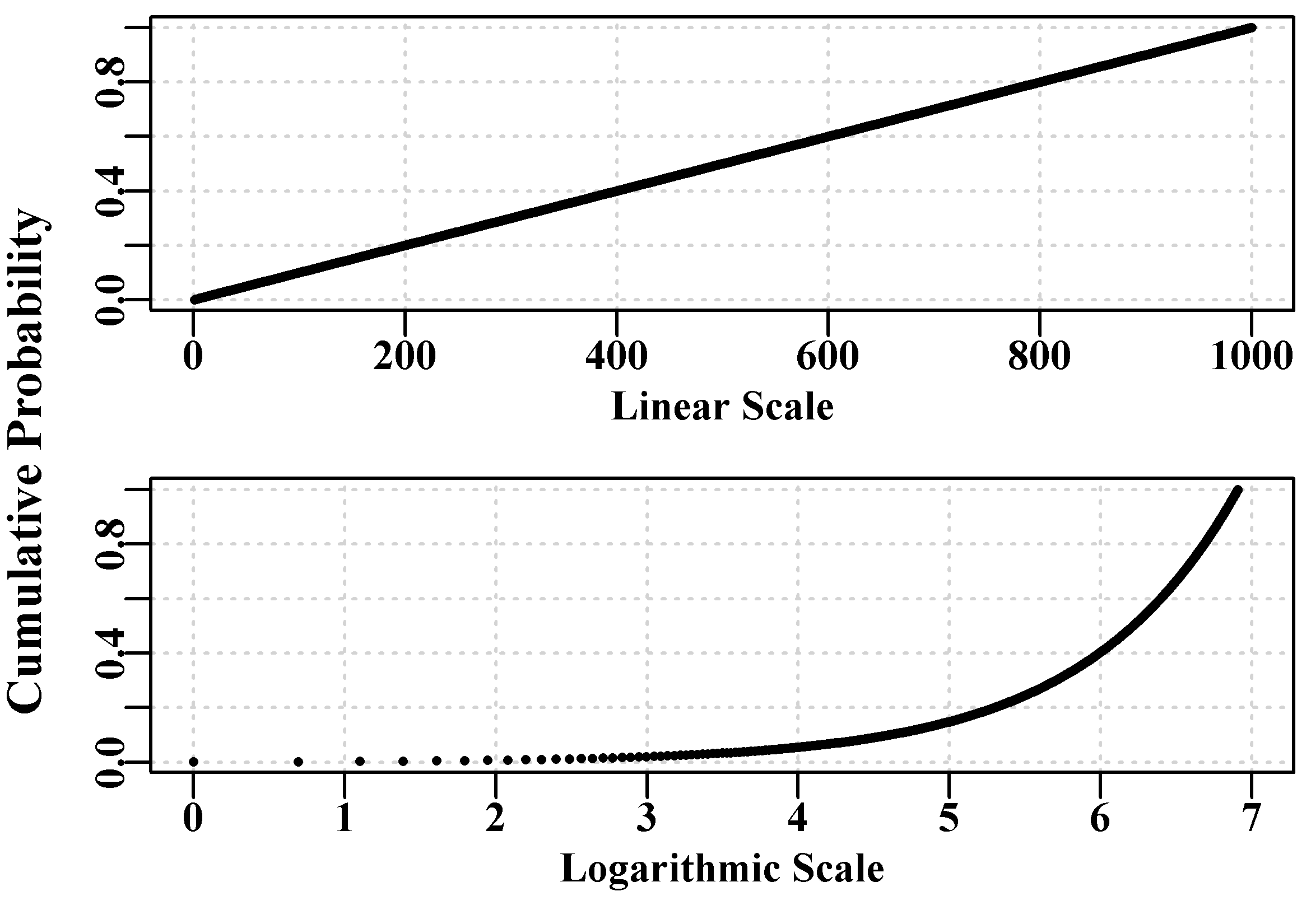
Figure 4.24: A constant set of prior probabilities accumulated on a linear scale and on a log scale.
As fisheries models tend to be full of nonlinear relationships, the use of non-informative priors is controversial because a prior that is non-informative with respect to some parameters will most likely be informative toward others. While such influences may be unintentional, they cannot be ignored. The implication is that information may be included into a model in a completely unintentional manner, which is one source of controversy when discussing prior probabilities. If priors are to be used, then Punt and Hilborn’s (1997) exhortation to fully document their origin and properties is extremely sensible advice. We will examine the use of Bayesian methods in much more detail in the chapter On Uncertainty.
4.14 Concluding Remarks
The optimum method to use in any analytical situation depends largely on the objectives of the analysis. If all one wants to do is to find the optimum fit to a model, then it does not really matter whether one uses least squares, maximum likelihood, or Bayesian methods. Sometimes it can be easier to fit a model using least squares and then progress to using likelihoods or Bayesian methods to create confidence intervals and risk assessments.
Confidence intervals around model parameters and outputs can be generated using traditional asymptotic methods (guaranteed symmetric and, with strongly nonlinear models, only roughly approximate), using likelihood profiles or by integrating Bayesian posteriors (the two are obviously strongly related), or one can use bootstrapping or Monte Carlo techniques.
It is not the case that the more detailed areas of assessing the relative risks of alternative management options are only possible using Bayesian methods. Bootstrapping and Monte Carlo methods provide the necessary tools with which to conduct such work. The primary concern should be to define the objective of the analysis. However, it would be bad practice to fit a model and not give some idea of the uncertainty surrounding each parameter and the sensitivity of the model’s dynamics of the various input parameters.
Because there is no clear winner among the methodological approaches, if one has the time, it is a reasonable idea to use more than one approach (especially a comparison of likelihood profiles, Bayesian posteriors, and bootstrapping). Whether it is possible to have sufficient resources to enable a resource modeller the time to conduct such an array of analyses is a different but equally real problem. If significant differences are found, then it would be well to investigate the reasons behind them. If different procedures suggest significantly different answers, it could be that too much is being asked of the available data and different analyses would be warranted.